
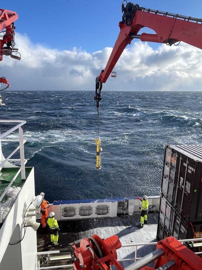
Anton und ich bringen soeben CTD-Cast Nummer 45 an das Tageslicht. Während wir gerade wieder einmal mit viel Enthusiasmus frisch gezapfte Flaschen durchschütteln, meine ich, ein nett gemeintes, aber deutliches Kopfschütteln bei Jamileh erkennen zu können, als sie uns ein Guten Morgen zulächelt. Das denken sich hier scheinbar alle: Bereits 45 CTD-Einsätze? Und viele davon an ein- und derselben Stelle? Warum das Ganze? Wir müssten das Wasser doch kennen, sobald wir es einmal „vermessen“ haben, oder? Naja, irgendwie schon.

„Unsere“ CTD, von den Biologen bevorzugt auch „Wasserschöpfer“ genannt, wird seitlich aus dem Hangar herausgefahren, herabgelassen und misst in der Basisversion quasi kontinuierlich (mit 24 Hz) Leitfähigkeit (Salzgehalt), Temperatur und Druck (Tiefe) (Conductivity, Temperature, Depth), idealerweise hinunter bis zum Meeresboden. Darüber hinaus werden Sauerstoffgehalt und Fluoreszenz gemessen, was eine Abschätzung der biologischen Produktivität ermöglicht (siehe Blogeinträge zu „Mikrokreaturen“ von Nicole und Manfred). Als praktische Zugabe können mithilfe der 24 Niskin-Flaschen Wasserproben in verschiedenen Tiefen genommen werden (Manfred ist da nebenbei bemerkt mit Abstand unser bester Kunde).
Für Ozeanographen sind aber vor allem die kontinuierlichen Messungen von Temperatur und Salzgehalt von entscheidender Bedeutung, da wir daraus z.B. ableiten können, wie stabil das Wasser geschichtet ist oder woher Wassermassen und geostrophische Strömungen kommen. Dies sind wichtige Informationen, die Rahmenbedingungen darstellen, die das lokale Ökosystem stark beeinflussen. Um eine möglichst hohe Genauigkeit der physikalischen Messungen zu erreichen, nehme ich auch selbst Wasserproben, allerdings „nur“ zur späteren Kalibrierung der verschiedenen Sensoren und nicht zur Analyse der darin enthaltenen kuriosen Lebewesen.

Die meisten Einsätze wurden bisher in Küstennähe in einer Tiefe von 1500 Metern gefahren. Die folgende Abbildung zeigt eines unserer wertvollen Tiefseeprofile bis in eine Tiefe von fast 3300 Metern. Hier bilden die obersten 100m die so genannte „Deckschicht“ (Mixed Layer), in welcher alle gemessenen Größen durch den Wind gut durchmischt sind. . Wir beobachten, dass die Tiefe der Deckschicht variiert, aber grundsätzlich – wie für die Wintermonate in diesen Breiten typisch – relativ mächtig ist. An unserer ersten Station betrug die Deckschichttiefe sogar ca. 200 Meter!

Temperatur (rot), Salz (blau), Sauerstoff (gelb) als auch Chlorophyll (grün) zeichnen praktisch vertikale Linien in das Diagramm. Interessanterweise bildet sich genau an bzw. unter der Deckschicht häufig ein Maximum an Chlorophyll, welches als Indikator für das Vorkommen von Phytoplankton dient (siehe wieder Nicoles und Manfreds Blog-Eintrag). Obwohl Phytoplankton grundsätzlich autotroph, also auf Sonnenlicht angewiesen ist, kann es in dieser recht Tiefen Schicht mit sehr wenig Sonnenlicht überleben. Ein Grund dafür ist der erhöhte Nährstoffgehalt in tieferen Schichten.
Darüber hinaus bildet die Pyknokline direkt unterhalb der Deckschicht eine starke physikalische Barriere für vertikale Vermischung und kann Organismen, die selbst nicht aktiv schwimmen können, praktisch „einsperren“. Die Pyknokline ist die Schicht, in der die Dichte des Wassers mit der Tiefe (hier aufgrund des Temperaturgradienten) sehr schnell zunimmt. Diese Schichten beherbergen eine hohe Spannbreite an Temperatur- und Salzgehalten und werden auch Zentralwasser genannt.
Um Wassermassen zu identifizieren, werden Temperaturen und Salzgehalte in einem sogenannten „T-S Diagramm“ (wie in Abbildung 4) gegeneinander aufgetragen. In unserem Beispiel sieht man gut, dass das Wasser rund um Madeira zu einem großen Teil aus Nordatlantischem Zentralwasser (Eastern North Atlantic Central Water) besteht. Dieses dominiert die Pyknokline im großen Nordatlantischen Wirbel und ist deutlich salzhaltiger als im Südatlantik (vgl. Eastern South Atlantic Central Water). In unserem Profil Nummer 41 (Abbildung 3) fällt aber noch etwas anderes ins Auge. Auf etwa 1100 Metern Tiefe zeigt sich eine Nase mit noch einmal deutlich erhöhtem Salzgehalt, die nicht so recht zum linear verlaufenden Zentralwasser zu passen scheint. Hier macht sich der Einfluss des Mittelmeerwassers (MW) bemerkbar, welches aufgrund der überwiegend starken Verdunstung bei gleichzeitig wenig Niederschlag im Mittelmeerraum besonders hohe Salzgehalte mit sich bringt. Aufgrund dieses hohen Salzgehaltes manifestiert es sich trotz der warmen Temperaturen in größeren Tiefen um typischerweise 1100-1200 Meter. Wir sehen im T-S Diagramm aber auch, dass das Mittelmeerwasser im Süden von Madeira bereits etwas durchmischter, also weniger warm und salzhaltig als direkt am Ausgang des Mittelmeeres ist. Noch tiefer, was wir insbesondere bei unseren ausgedehnteren CTD-Stationen bis auf 3000 Meter und mehr gut beobachten können, findet sich das berühmte Nordatlantische Tiefenwasser (North Atlantic Deep Water). Dieses wird unter anderem durch Tiefenkonvektion im Nordatlantik gebildet und spielt eine zentrale Rolle für die globale thermohaline Zirkulation, und die gesamte Klimadynamik. Es ist für Tiefenwasser relativ „jung“ und damit reich an Sauerstoff (wir sagen gerne „gut ventiliert“) und bildet einen Kontrast zum Sauerstoffminimum, welches wir hier um Madeira auf etwa 800-900 Metern beobachten. Diese Minimumzone entsteht durch Respiration des abgesunkenen organischen Materials, z.B. von dem sonnenlichtabhängigen Phytoplankton in den obersten ~150 Metern. Im Vergleich mit den großen bekannten Sauerstoffminimumzonen im subtropischen Ost-Atlantik und -Pazifik, ist jedoch noch vergleichsweise reichlich Sauerstoff vorhanden.

Nun kennen wir das Profil einer CTD-Station etwas genauer. Im Grunde ist dieses sogar ziemlich repräsentativ für die übrigen 44. Die Frage, warum Anton und ich wie die Wahnsinnigen weiter „CTDs fahren“, bleibt also noch unbeantwortet. Wenn wir jedoch genauer hinschauen, sehen wir, dass die Temperatur- und Salzprofile nicht komplett „glatt“ verlaufen. Tatsächlich entdecken wir kleine wellenförmige Abweichungen. Messungenauigkeiten? Nein. Es sind interne Wellen, die die Profile lebendig machen. Interne Wellen können in jedem stratifizierten Medium auftreten, also Fluide, in denen die Dichte nicht konstant ist. Es gibt zwei rückstellende Kräfte, die auf interne Wellen im Ozean wirken: Gravitation und die Corioliskraft. Hauptantriebe für interne Wellen sind die Gezeiten (wie Ebbe und Flut), dicht gefolgt von Wind. Wir wissen, dass interne Wellen eine entscheidende Rolle für den Energietransport im Ozean spielen. Wie gewöhnliche Oberflächenwellen, können auch interne Wellen brechen. Wenn sie das tun, findet Vermischung statt. Das wiederum kann Nährstoffe transportieren und dadurch die biologische Produktivität beeinflussen. Die Wechselwirkung von internen Wellen mit Topographie (d.h. Inseln wie Madeira) und Strömungen ist sehr komplex und noch nicht vollumfänglich verstanden. Durch eine hohe Anzahl an Stationen zu verschiedenen Zeiten (und Gezeitenstadien) erhalten wir eine bessere räumliche und zeitliche Auflösung des internen Wellenfeldes und können die Prozesse besser verstehen. Deswegen sind wir z.B. Fans von sogenannten „Jo-Jo-CTDs“. Wie bei einem echten Jo-Jo fahren wir die CTD an ein- und derselben Stelle mehrfach direkt hintereinander auf- und ab.

In der obigen Abbildung haben wir sechs direkt aufeinander folgende Profile eines „Jo-Jos“ übereinander geplottet. Man erkennt, dass die Profile auf manchen Tiefen mehr voneinander abweichen, und auf anderen wieder nicht (Knotenpunkte). Den imposantesten Einfluss nehmen interne Wellen auf die Deckschichttiefe, diese kann alleine dadurch innerhalb von Minuten um mehrere zehn Meter variieren.
Besonderer Nervenkitzel kommt auf, wenn zur „Eddy-Jagd“ aufgerufen wird. Das klingt jetzt martialischer, als es gemeint ist. Eddies sind ozeanische Wirbel, die rund um Madeira einen Durchmesser von ca. 50 Kilometern erreichen, mit der Topographie (Inseln) sowie internen Wellen interagieren und bekanntermaßen die Biodiversität beeinflussen können. Sie entstehen über einen Zeitraum von Tagen / Wochen und sind leider kaum vorhersagbar. Daher checken wir täglich Satelliten- und Modelldaten für die Region, um ein mögliches Feature zu identifizieren, und falls möglich, in situ mit dem Schiff zu beproben. Starke Eddies können ein Signal in der Meereshöhe, den Oberflächentemperaturen und im Chlorophyll erzeugen.
Unsere Kollegen vom Ozeanographischen Institut Madeira unterstützen uns vor Ort mit regionalen Satelliten- und Modelldaten (siehe https://oomdata.arditi.pt/msm126/ ). Es ist insgesamt beeindruckend, wie gut die Zusammenarbeit an Bord und darüber hinaus funktioniert! In der Nacht vom 13. auf den 14. Februar fand bereits eine „Eddy-Jagd“ statt. Allerdings war das Satellitensignal schwach und dementsprechend konnten wir vor Ort mit unserem schiffseigenen ADCP (das Ozeanströmungen bis in knapp 1000 Meter Tiefe misst) keinen starken, kohärenten Wirbel nachweisen.(Randbemerkung: Es wurde dabei aber ein anderes spannendendes feature (mutmaßlich eine kräftige interne Welle) in der Deckschicht ausgemacht, welches wir nun analysieren.)

In einem der nächsten Blogeinträge wollen wir euch beweisen, dass unsere lieb gewonnene CTD dank raffinierter Tunings, unter anderem mit hochauflösenden Kamerasystemen, rein „objektiv“ etwas ganz Besonderes ist. Dann klären wir auf, warum auch Anton, obwohl er kein physikalischer Ozeanograph ist, gerne „Jo-Jos“ fährt, und es gibt endlich wieder Fotos von Wassertierchen!
Viele Grüße von Bord der MARIA S. MERIAN,
Marco Schulz und Anton Theileis


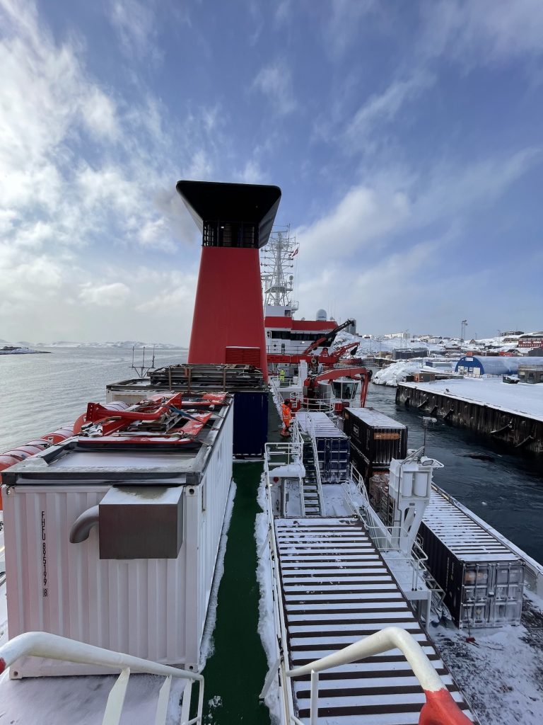
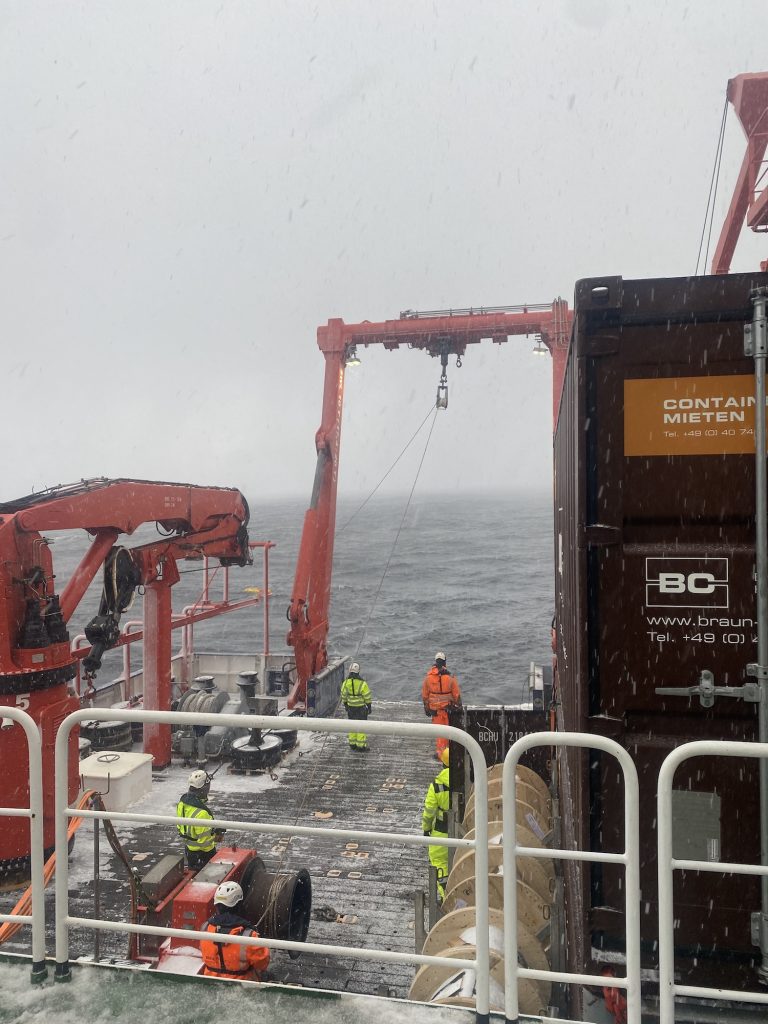
After a slight delay of the Maria S. Merian caused by late-arriving containers our research cruise MSM142 finally got underway. By last Tuesday (24.03.2026), the full scientific team had arrived in Nuuk, the capital of Greenland, and the ship reached port on Wednesday (25.03.2026) morning. That same day, scientists and technicians moved on board and immediately began preparations, assembling and testing our instruments. Although the mornings on Wednesday and Thursday were grey and overcast, the afternoons cleared up beautifully. This gave us valuable time to organize equipment on deck and store empty boxes back into the containers before departure.
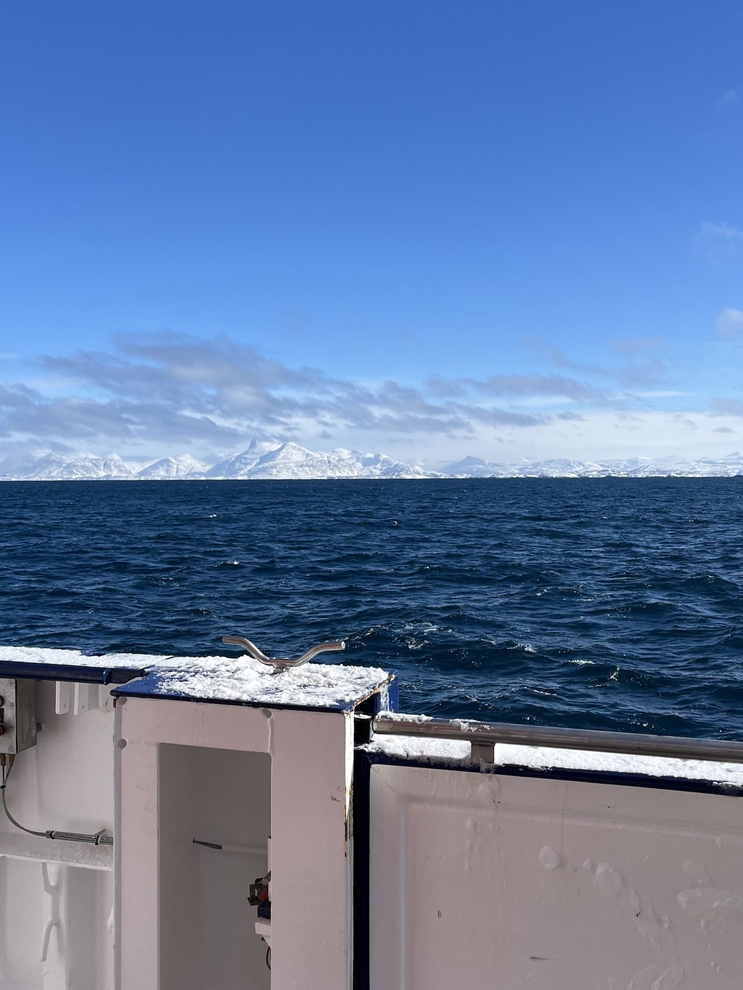
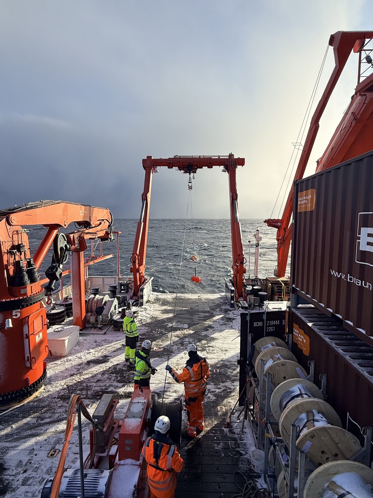
Given the forecast of harsh conditions outside the fjord, we carried out the mandatory safety drill while still in harbour. This included practicing emergency procedures and boarding the lifeboat. After completing border control, we were finally ready to leave Nuuk. We set sail on March 27th, heading into the Labrador Sea to begin our mission. Even before starting scientific operations, we tested the setup for deploying our gliders without releasing them during the transit out of the fjord. Once we reached open waters, we were met by high waves the following morning. For some on board, this was their first experience under such rough sea conditions. Seasickness quickly became a challenge for a few, while scientific work had to be temporarily postponed due to the strong winds and sea conditions. Together with the crew, we discussed how best to adapt our measurement plans to the given weather conditions. On March 29th, we were finally able to begin our scientific program with the first CTD deployment. A CTD is an instrument used to measure conductivity, temperature, and depth, which are key parameters for understanding ocean structure.
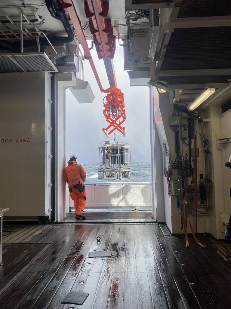
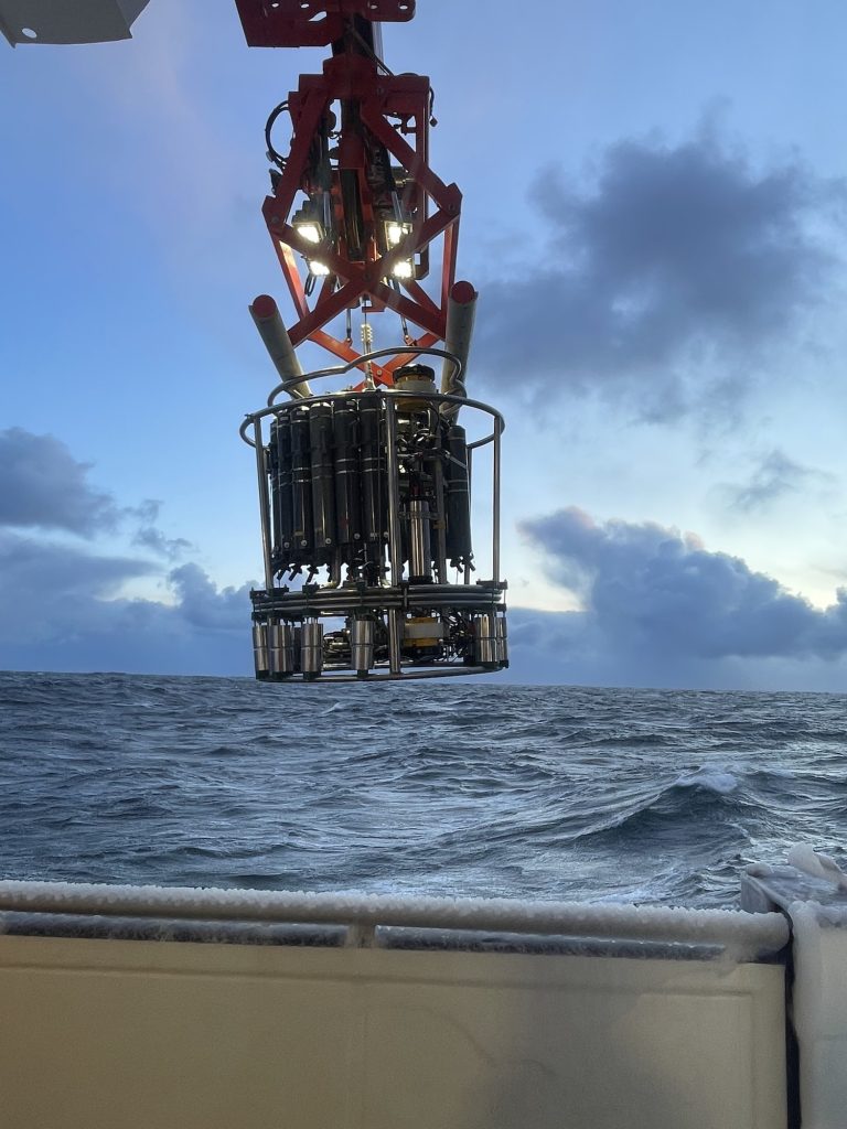
During the following night, we continued with additional CTD stations and successfully recovered two moorings: DSOW 3 and DSOW 4, located south of Greenland. These moorings carry instruments at various depths that measure velocity, temperature, and salinity. DSOW 4 was redeployed on the same day, while DSOW 3 followed the next day. In addition, the bottles attached to the CTD’s rosette can be used to collect water samples from any desired depth. These samples can be used, for example, to determine the oxygen content, nutrient levels, and organic matter.
Both are part of the OSNAP array, a network of moorings spanning the subpolar North Atlantic. On these moorings are a few instruments, for example microcats which measure temperature, pressure and salinity.
We then conducted around 25 CTD stations spaced approximately 3 nautical miles apart across an Irminger ring identified from satellite data. This high-resolution sampling was necessary to capture the structure of an Irminger Ring, which had a radius of about 12 km wide.
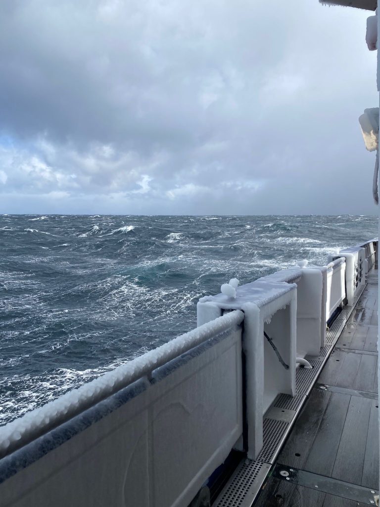
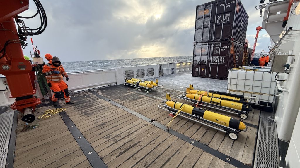
The days leading up to April 2nd were marked by very rough weather conditions. Life on board became both challenging and, at times, unintentionally entertaining sliding chairs were not uncommon. During the night from April 1st to April 2nd, winds reached 11 Beaufort with gusts up to 65 knots, forcing us to pause our measurements. Fortunately, conditions improved by morning, allowing us to resume our work. As well as with the help of the crew we had to adapt to the harsh weather conditions to continue our scientific work. On the 3rd of April, we were able to deploy a few gliders and one float. An ocean glider is an autonomous underwater Vehicle, which you can steer remotely and send to different locations, while it is measuring oceanographic key parameters.
This research cruise focuses on understanding small-scale processes in the ocean and their connection to the spring bloom, an essential phase in marine ecosystem in subpolar regions. Despite the challenging start, we have already gathered valuable data and look forward to the weeks ahead in the Labrador Sea.
Despite their dramatic name, false killer whales aren’t an orca species. These animals are dolphins—members of the same extended family as the iconic “killer whale” (Orcinus orca). Compared to their namesake counterparts, these marine mammals are far less well-known than our ocean’s iconic orcas.
Let’s dive in and take a closer look at false killer whales—one of the ocean’s most social, yet lesser-known dolphin species.
Appearance and anatomy
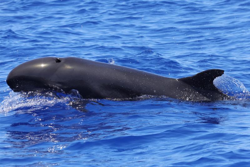
False killer whales (Pseudorca crassidens) are among the largest members of the dolphin family (Delphinidae). Adults can grow up to 20 feet long and weigh between 1,500 and 3,000 pounds, though some individuals have been recorded weighing even more. For comparison, that’s roughly double the size of a bottlenose dolphin—and slightly larger than a typical sedan.
These animals are incredibly powerful swimmers with long, torpedo-shaped bodies that help them move efficiently through the open ocean in search of prey. Their skull structure is what earned them their name, as their head shape closely resembles that of orcas. With broad, rounded heads, muscular jaws and large cone-shaped teeth, early scientists were fascinated by the similarities between these two marine mammal species.
Although their heads may look somewhat like those of orcas, there are several ways to distinguish false killer whales from their larger namesake counterparts.
One of the most noticeable differences has to do with their coloration. While orcas are known for their iconic black-and-white pattern with paler underbellies, alternatively, false killer whales are typically a uniform dark gray to black in color—almost as if a small orca decided to roll around in the dirt. If you’ve ever seen the animated Disney classic 101 Dalmatians, the difference is a bit like when the puppies roll in soot to disguise themselves as labradors instead of showing their usual black-and-white spots.
Their teeth also present a differentiator. The scientific name Pseudorca crassidens translates almost literally to “thick-toothed false orca,” a nod to their sturdy, cone-shaped teeth that help these animals capture prey. Orcas tend to have more robust, bulbous heads, while false killer whales appear slightly narrower and more streamlined.
Behavior and diet
False killer whales are both highly efficient hunters and deeply social animals. It’s not unusual to see them hunting together both in small pods and larger groups as they pursue prey like fish and squid.
Scientists have even observed false killer whales sharing food with each other, a behavior that is very unusual for marine mammals. While some dolphin and whale species work together to pursue prey, they rarely actively share food. The sharing of food among false killer whales spotlights the strong social bonds within their pods. Researchers believe these tight-knit social connections help false killer whales thrive in offshore environments where they’re always on the move.
Maintaining these close bonds and coordinating successful hunts requires constant effective communication, and this is where false killer whales excel. Like other dolphins, they produce a variety of sounds like whistles and clicks to stay connected with their pod and locate prey using echolocation. In the deep offshore waters where they live, sound often becomes more important than sight, since sound travels much farther underwater than light.
Where they live
False killer whales are highly migratory and travel long distances throughout tropical and subtropical waters around the world. They prefer deeper waters far offshore, and this pelagic lifestyle can make them more difficult for scientists to study than many coastal dolphin species.
However, there are a few places where researchers have been able to learn more about them—including the waters surrounding the Hawaiian Islands.
Scientists have identified three distinct groups of false killer whales in and around Hawaii, but one well-studied group stays close to the main Hawaiian Islands year-round. Unfortunately, researchers estimate that only about 140 individuals remained in 2022, with populations expected to decline without action to protect them. This is exactly why this group is listed as endangered under the U.S. Endangered Species Act and is considered one of the most vulnerable marine mammal populations in U.S. waters.
Never Miss An Update
Sign up for Ocean Conservancy text messages today.
Current threats to survival
False killer whales are currently listed as Near Threatened on the IUCN Red List. From climate change-induced ocean acidification and harmful algal blooms to marine debris and fishing bycatch, false killer whales face the same mounting pressures that are impacting marine ecosystems around the world. As their prey becomes scarce due to increasing threats, populations of top predators like these decline, serving as a powerful signal that the ocean’s overall health is in critical need of protection.
Here at Ocean Conservancy, we’re working daily to confront these threats head-on and protect the ecosystems and wildlife we all cherish so dearly. But we can’t do it without you. Support from ocean lovers is what powers our work to protect our ocean, and right now, our planet needs all the help it can get. Visit Ocean Conservancy’s Action Center today and join our movement to create a better future for our ocean, forever and for everyone.
The post All About False Killer Whales appeared first on Ocean Conservancy.
https://oceanconservancy.org/blog/2026/03/31/false-killer-whales/
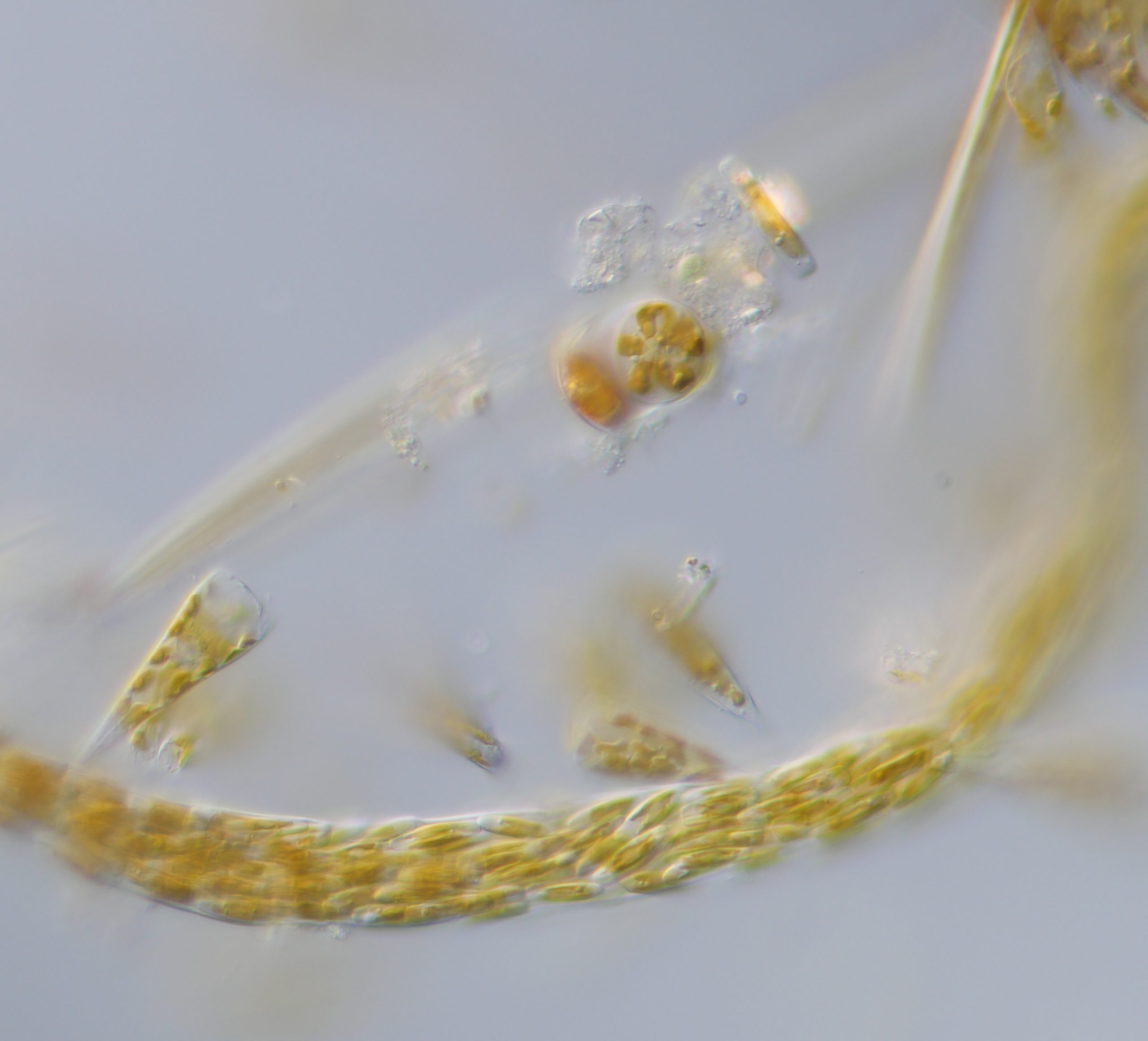
A lot has happened in the meantime: I became an Associate Professor at the University of Southern Denmark, we all lived through the Corona period, then slowly adjusted to the post‑pandemic stability, only to find ourselves again in turbulent political times. I am now affiliated with the Marine Research Center in Kerteminde, a beautiful coastal town on the island of Fyn. My plan is to share small updates on my research and activities every now and then. So let’s start with yesterday’s sampling trip for benthic phytoplankton, carried out by my colleague, Prof. Kazumasa Oguri. The sampling will help prepare for the first‑semester bachelor students who will join his small but fascinating project. This project is all about the benthic diatoms that form dense, photosynthetic communities on tidal‑flat sediments. Their daytime oxygen production enriches the sediment surface and allows oxygen to penetrate deeper, supporting diverse organisms that rely on aerobic respiration. The project will explore how oxygen distribution and oxygen production/consumption in sediments change under different light conditions (day, night, sunrise/sunset). The team will incubate benthic diatom communities in jars and measure oxygen profiles using an oxygen imaging system under controlled light regimes.
Yesterday, we visited several potential sampling sites where students can carry out their fieldwork. I encourage all PIs in our group to define at least one small project related to Kerteminde Fjord, where our laboratories are located. Over time, I hope we can build a more integrated dataset describing the marine and coastal ecosystems of the area.
Another activity currently in preparation is a project on marine invasive species in Kerteminde, which will feed into a course I will run in July and a master’s thesis project. More will come later.
Let’s hope for a more continuous blog from here on, keeping track of our activities, with or without jellyfish!

After a Slow Start on Climate, Zohran Mamdani Faces Scrutiny Over Parks Budget and Environmental Promises
Who Loses in the Trump Administration’s $1 Billion ‘Deal’ to Abandon Offshore Wind?
Minneapolis Activists Launch Hunger Strike to Protest Polluting Trash Incinerator
-
Climate Change8 months ago
Guest post: Why China is still building new coal – and when it might stop
-
Greenhouse Gases8 months ago
Guest post: Why China is still building new coal – and when it might stop
-

 Greenhouse Gases2 years ago
嘉宾来稿:满足中国增长的用电需求 光伏加储能“比新建煤电更实惠”
-
Climate Change2 years ago
Bill Discounting Climate Change in Florida’s Energy Policy Awaits DeSantis’ Approval
-

 Climate Change2 years ago
嘉宾来稿:满足中国增长的用电需求 光伏加储能“比新建煤电更实惠”
-
Climate Change Videos2 years ago
The toxic gas flares fuelling Nigeria’s climate change – BBC News
-

 Renewable Energy6 months ago
Sending Progressive Philanthropist George Soros to Prison?
-

 Carbon Footprint2 years ago
US SEC’s Climate Disclosure Rules Spur Renewed Interest in Carbon Credits