
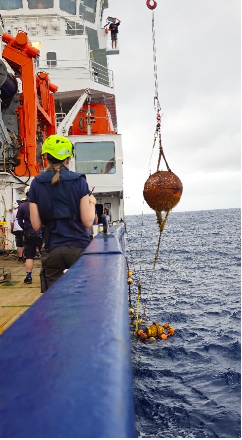
Anton und ich bringen soeben CTD-Cast Nummer 45 an das Tageslicht. Während wir gerade wieder einmal mit viel Enthusiasmus frisch gezapfte Flaschen durchschütteln, meine ich, ein nett gemeintes, aber deutliches Kopfschütteln bei Jamileh erkennen zu können, als sie uns ein Guten Morgen zulächelt. Das denken sich hier scheinbar alle: Bereits 45 CTD-Einsätze? Und viele davon an ein- und derselben Stelle? Warum das Ganze? Wir müssten das Wasser doch kennen, sobald wir es einmal „vermessen“ haben, oder? Naja, irgendwie schon.

„Unsere“ CTD, von den Biologen bevorzugt auch „Wasserschöpfer“ genannt, wird seitlich aus dem Hangar herausgefahren, herabgelassen und misst in der Basisversion quasi kontinuierlich (mit 24 Hz) Leitfähigkeit (Salzgehalt), Temperatur und Druck (Tiefe) (Conductivity, Temperature, Depth), idealerweise hinunter bis zum Meeresboden. Darüber hinaus werden Sauerstoffgehalt und Fluoreszenz gemessen, was eine Abschätzung der biologischen Produktivität ermöglicht (siehe Blogeinträge zu „Mikrokreaturen“ von Nicole und Manfred). Als praktische Zugabe können mithilfe der 24 Niskin-Flaschen Wasserproben in verschiedenen Tiefen genommen werden (Manfred ist da nebenbei bemerkt mit Abstand unser bester Kunde).
Für Ozeanographen sind aber vor allem die kontinuierlichen Messungen von Temperatur und Salzgehalt von entscheidender Bedeutung, da wir daraus z.B. ableiten können, wie stabil das Wasser geschichtet ist oder woher Wassermassen und geostrophische Strömungen kommen. Dies sind wichtige Informationen, die Rahmenbedingungen darstellen, die das lokale Ökosystem stark beeinflussen. Um eine möglichst hohe Genauigkeit der physikalischen Messungen zu erreichen, nehme ich auch selbst Wasserproben, allerdings „nur“ zur späteren Kalibrierung der verschiedenen Sensoren und nicht zur Analyse der darin enthaltenen kuriosen Lebewesen.

Die meisten Einsätze wurden bisher in Küstennähe in einer Tiefe von 1500 Metern gefahren. Die folgende Abbildung zeigt eines unserer wertvollen Tiefseeprofile bis in eine Tiefe von fast 3300 Metern. Hier bilden die obersten 100m die so genannte „Deckschicht“ (Mixed Layer), in welcher alle gemessenen Größen durch den Wind gut durchmischt sind. . Wir beobachten, dass die Tiefe der Deckschicht variiert, aber grundsätzlich – wie für die Wintermonate in diesen Breiten typisch – relativ mächtig ist. An unserer ersten Station betrug die Deckschichttiefe sogar ca. 200 Meter!

Temperatur (rot), Salz (blau), Sauerstoff (gelb) als auch Chlorophyll (grün) zeichnen praktisch vertikale Linien in das Diagramm. Interessanterweise bildet sich genau an bzw. unter der Deckschicht häufig ein Maximum an Chlorophyll, welches als Indikator für das Vorkommen von Phytoplankton dient (siehe wieder Nicoles und Manfreds Blog-Eintrag). Obwohl Phytoplankton grundsätzlich autotroph, also auf Sonnenlicht angewiesen ist, kann es in dieser recht Tiefen Schicht mit sehr wenig Sonnenlicht überleben. Ein Grund dafür ist der erhöhte Nährstoffgehalt in tieferen Schichten.
Darüber hinaus bildet die Pyknokline direkt unterhalb der Deckschicht eine starke physikalische Barriere für vertikale Vermischung und kann Organismen, die selbst nicht aktiv schwimmen können, praktisch „einsperren“. Die Pyknokline ist die Schicht, in der die Dichte des Wassers mit der Tiefe (hier aufgrund des Temperaturgradienten) sehr schnell zunimmt. Diese Schichten beherbergen eine hohe Spannbreite an Temperatur- und Salzgehalten und werden auch Zentralwasser genannt.
Um Wassermassen zu identifizieren, werden Temperaturen und Salzgehalte in einem sogenannten „T-S Diagramm“ (wie in Abbildung 4) gegeneinander aufgetragen. In unserem Beispiel sieht man gut, dass das Wasser rund um Madeira zu einem großen Teil aus Nordatlantischem Zentralwasser (Eastern North Atlantic Central Water) besteht. Dieses dominiert die Pyknokline im großen Nordatlantischen Wirbel und ist deutlich salzhaltiger als im Südatlantik (vgl. Eastern South Atlantic Central Water). In unserem Profil Nummer 41 (Abbildung 3) fällt aber noch etwas anderes ins Auge. Auf etwa 1100 Metern Tiefe zeigt sich eine Nase mit noch einmal deutlich erhöhtem Salzgehalt, die nicht so recht zum linear verlaufenden Zentralwasser zu passen scheint. Hier macht sich der Einfluss des Mittelmeerwassers (MW) bemerkbar, welches aufgrund der überwiegend starken Verdunstung bei gleichzeitig wenig Niederschlag im Mittelmeerraum besonders hohe Salzgehalte mit sich bringt. Aufgrund dieses hohen Salzgehaltes manifestiert es sich trotz der warmen Temperaturen in größeren Tiefen um typischerweise 1100-1200 Meter. Wir sehen im T-S Diagramm aber auch, dass das Mittelmeerwasser im Süden von Madeira bereits etwas durchmischter, also weniger warm und salzhaltig als direkt am Ausgang des Mittelmeeres ist. Noch tiefer, was wir insbesondere bei unseren ausgedehnteren CTD-Stationen bis auf 3000 Meter und mehr gut beobachten können, findet sich das berühmte Nordatlantische Tiefenwasser (North Atlantic Deep Water). Dieses wird unter anderem durch Tiefenkonvektion im Nordatlantik gebildet und spielt eine zentrale Rolle für die globale thermohaline Zirkulation, und die gesamte Klimadynamik. Es ist für Tiefenwasser relativ „jung“ und damit reich an Sauerstoff (wir sagen gerne „gut ventiliert“) und bildet einen Kontrast zum Sauerstoffminimum, welches wir hier um Madeira auf etwa 800-900 Metern beobachten. Diese Minimumzone entsteht durch Respiration des abgesunkenen organischen Materials, z.B. von dem sonnenlichtabhängigen Phytoplankton in den obersten ~150 Metern. Im Vergleich mit den großen bekannten Sauerstoffminimumzonen im subtropischen Ost-Atlantik und -Pazifik, ist jedoch noch vergleichsweise reichlich Sauerstoff vorhanden.

Nun kennen wir das Profil einer CTD-Station etwas genauer. Im Grunde ist dieses sogar ziemlich repräsentativ für die übrigen 44. Die Frage, warum Anton und ich wie die Wahnsinnigen weiter „CTDs fahren“, bleibt also noch unbeantwortet. Wenn wir jedoch genauer hinschauen, sehen wir, dass die Temperatur- und Salzprofile nicht komplett „glatt“ verlaufen. Tatsächlich entdecken wir kleine wellenförmige Abweichungen. Messungenauigkeiten? Nein. Es sind interne Wellen, die die Profile lebendig machen. Interne Wellen können in jedem stratifizierten Medium auftreten, also Fluide, in denen die Dichte nicht konstant ist. Es gibt zwei rückstellende Kräfte, die auf interne Wellen im Ozean wirken: Gravitation und die Corioliskraft. Hauptantriebe für interne Wellen sind die Gezeiten (wie Ebbe und Flut), dicht gefolgt von Wind. Wir wissen, dass interne Wellen eine entscheidende Rolle für den Energietransport im Ozean spielen. Wie gewöhnliche Oberflächenwellen, können auch interne Wellen brechen. Wenn sie das tun, findet Vermischung statt. Das wiederum kann Nährstoffe transportieren und dadurch die biologische Produktivität beeinflussen. Die Wechselwirkung von internen Wellen mit Topographie (d.h. Inseln wie Madeira) und Strömungen ist sehr komplex und noch nicht vollumfänglich verstanden. Durch eine hohe Anzahl an Stationen zu verschiedenen Zeiten (und Gezeitenstadien) erhalten wir eine bessere räumliche und zeitliche Auflösung des internen Wellenfeldes und können die Prozesse besser verstehen. Deswegen sind wir z.B. Fans von sogenannten „Jo-Jo-CTDs“. Wie bei einem echten Jo-Jo fahren wir die CTD an ein- und derselben Stelle mehrfach direkt hintereinander auf- und ab.

In der obigen Abbildung haben wir sechs direkt aufeinander folgende Profile eines „Jo-Jos“ übereinander geplottet. Man erkennt, dass die Profile auf manchen Tiefen mehr voneinander abweichen, und auf anderen wieder nicht (Knotenpunkte). Den imposantesten Einfluss nehmen interne Wellen auf die Deckschichttiefe, diese kann alleine dadurch innerhalb von Minuten um mehrere zehn Meter variieren.
Besonderer Nervenkitzel kommt auf, wenn zur „Eddy-Jagd“ aufgerufen wird. Das klingt jetzt martialischer, als es gemeint ist. Eddies sind ozeanische Wirbel, die rund um Madeira einen Durchmesser von ca. 50 Kilometern erreichen, mit der Topographie (Inseln) sowie internen Wellen interagieren und bekanntermaßen die Biodiversität beeinflussen können. Sie entstehen über einen Zeitraum von Tagen / Wochen und sind leider kaum vorhersagbar. Daher checken wir täglich Satelliten- und Modelldaten für die Region, um ein mögliches Feature zu identifizieren, und falls möglich, in situ mit dem Schiff zu beproben. Starke Eddies können ein Signal in der Meereshöhe, den Oberflächentemperaturen und im Chlorophyll erzeugen.
Unsere Kollegen vom Ozeanographischen Institut Madeira unterstützen uns vor Ort mit regionalen Satelliten- und Modelldaten (siehe https://oomdata.arditi.pt/msm126/ ). Es ist insgesamt beeindruckend, wie gut die Zusammenarbeit an Bord und darüber hinaus funktioniert! In der Nacht vom 13. auf den 14. Februar fand bereits eine „Eddy-Jagd“ statt. Allerdings war das Satellitensignal schwach und dementsprechend konnten wir vor Ort mit unserem schiffseigenen ADCP (das Ozeanströmungen bis in knapp 1000 Meter Tiefe misst) keinen starken, kohärenten Wirbel nachweisen.(Randbemerkung: Es wurde dabei aber ein anderes spannendendes feature (mutmaßlich eine kräftige interne Welle) in der Deckschicht ausgemacht, welches wir nun analysieren.)

In einem der nächsten Blogeinträge wollen wir euch beweisen, dass unsere lieb gewonnene CTD dank raffinierter Tunings, unter anderem mit hochauflösenden Kamerasystemen, rein „objektiv“ etwas ganz Besonderes ist. Dann klären wir auf, warum auch Anton, obwohl er kein physikalischer Ozeanograph ist, gerne „Jo-Jos“ fährt, und es gibt endlich wieder Fotos von Wassertierchen!
Viele Grüße von Bord der MARIA S. MERIAN,
Marco Schulz und Anton Theileis


By Qi-Fan Wu (Niels Bohr Institutet, University of Copenhagen)
During our journey, we saw many beautiful cloud patterns while looking outside the METEOR! Even though people do not always pay attention to them, clouds are among the most visible elements of the sky and naturally form part of our everyday background. And when we sailed away from the coastal region of Recife to the open ocean, the sky seemed to open up, allowing clouds to reveal their full variety and structure.
In climate modelling, clouds are one of the biggest sources of uncertainty. There is a famous saying in mathematics: “Mathematics is the queen of the sciences, number theory is the crown of mathematics, and the Goldbach Conjecture is the pearl on the crown.” The same idea can be applied to the study of clouds in Earth science. There is still no general macroscopic theory of clouds. Cloud physics is an absolutely fascinating topic, as it combines turbulence, stochastic processes, chemicals in the air, multiscale interactions within the Earth–atmosphere system, and a close connection to our daily weather.
In this blog entry, we would like to share some lovely photos of cloud patterns that we took on METEOR. Instead of serious systematic investigations, we focus on the basic cloud physics behind some typical cloud phenomena shown in these photos. These examples might provide something interesting to think about during our leisure time, even after returning to land. If nature is an artist, clouds are among its finest masterpieces, shaped by physical laws and stochastic processes.
What are clouds, and what is inside them? Clouds are made of many liquid water droplets and ice crystals inside the boundaries of the cloud. They are mostly air, with the many particles dispersed widely and more or less randomly throughout the cloud interiors [a]. The individual particles that make up a cloud are very, very small and not generally visible to the human eye.
When we look up from our research vessel METEOR and observe clouds, we first see their macroscopic structure: their overall shape, height, thickness, and organization across the sky. Broad, layered clouds often form through slow, large-scale ascent, while towering clouds with visible turrets reflect rapid rising motion in smaller air parcels. These visible forms are continuously shaped by moisture supply, cooling, turbulence, mixing with drier air, and precipitation, linking the large-scale atmospheric flow to the clouds we observe [a,b].
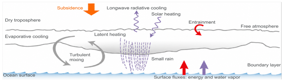
After leaving Recife, we entered a region typically influenced by the southeast trade winds of the tropical South Atlantic, where a vertically layered atmosphere, warm ocean conditions, and wind-driven mixing often promote a turbulent marine boundary layer. In Figure 1, the sky shows a layered cloudscape ranging from thin, high cirrostratus and altocumulus clouds to low cumulus and towering cumulonimbus clouds. These different forms reflect how the atmosphere organizes moisture, cooling, and vertical motion: broad layers are associated with gradual ascent, while the rising turrets of cumulus and cumulonimbus reveal stronger localized updrafts. Together, they illustrate the visible macroscopic structure of clouds, shaped by atmospheric motion and the microphysical processes occurring within them.
It should be noted that, in general, atmospheric temperature in the troposphere decreases with increasing altitude. Over the subtropical oceans, however, this is not the case. A relatively thin temperature-inversion layer lies above the subtropical marine boundary layer, within which temperature increases with height and the atmosphere is highly stable (Figure 2). Cloud occurrence above the marine boundary layer is relatively low in this region. The base of the trade-wind inversion is typically located at an altitude of approximately 1–2 km, separating the moist lower layer from the dry free troposphere [c].
This large-scale thermodynamic structure provides the environmental conditions under which clouds form and evolve. At the microscopic scale, however, clouds consist of particles: liquid water droplets, ice crystals, or a mixture of both. Clouds composed entirely of liquid droplets are commonly referred to as “warm clouds”, whereas clouds containing ice particles are classified as “cold clouds”. When liquid droplets and ice crystals coexist, the cloud is described as a mixed-phase cloud. However, the distinction between “warm” and “cold” clouds hinge on the phase of the particles, not on the temperature. The warm/cold distinction depends on the microphysical phase of the particles inside the cloud, which a normal naked eye observation cannot resolve.
Warm clouds consist of liquid water droplets spanning a range of sizes, from small haze droplets and cloud condensation nuclei to cloud droplets, drizzle drops, and raindrops (Figure 3). Cloud droplets typically form when water vapour condenses onto cloud condensation nuclei. Rainfall develops when some droplets grow much larger: larger droplets fall faster, collide with smaller droplets, and collect them. As a result, many small cloud droplets can combine to form fewer, larger drizzle drops and eventually raindrops [a]. This process approximately conserves the total liquid-water mass within the cloud, while transferring water from numerous small droplets to a much smaller number of large drops that are heavy enough to fall as rain.
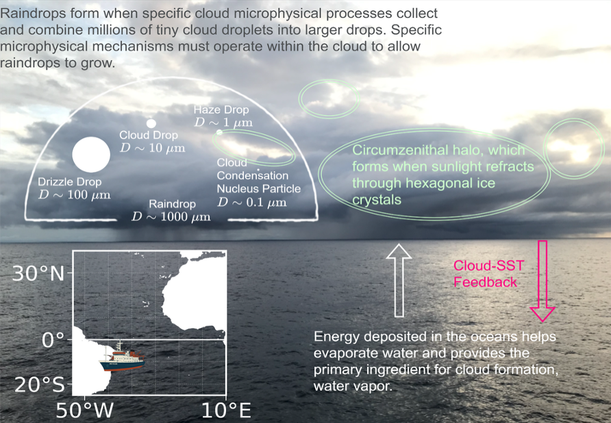
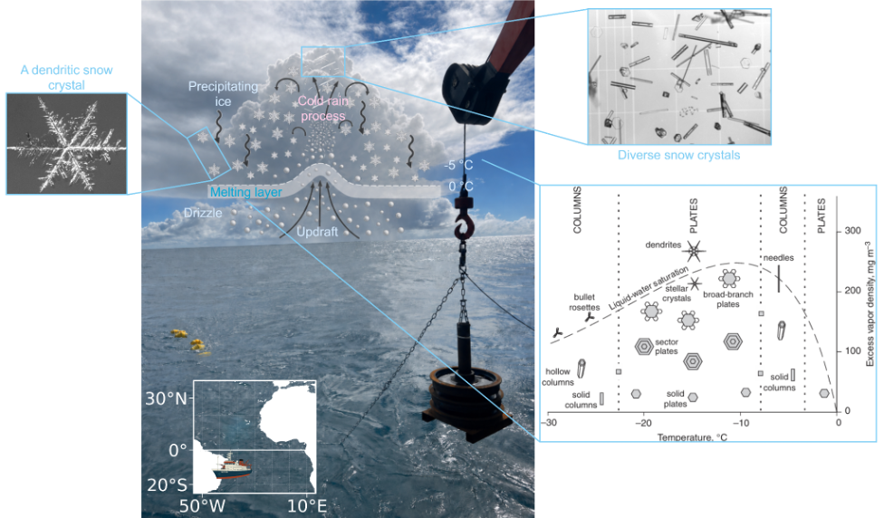
Cold clouds contain ice particles, either alone or together with supercooled liquid water droplets [a]. Unlike liquid droplets, which are nearly spherical because of surface tension, ice particles can develop a wide range of crystalline shapes, including plates, columns, needles, dendrites, and aggregates (Figure 4). Their shape depends mainly on temperature and ice supersaturation during growth by water-vapour deposition. As ice crystals become large enough to fall, they may collide and stick together to form snow aggregates, or collect supercooled droplets that freeze on contact, a process known as riming. The regular hexagonal structure of ice crystals can also produce optical phenomena such as halos, which form when sunlight is refracted or reflected by suitably oriented ice crystals in high-level clouds as shown in Figure 3. In mixed-phase clouds, uplift supports the growth of ice crystals at the expense of supercooled droplets. Once sufficiently large, the ice precipitates and may melt into rain or drizzle while falling through the melting layer (Figure 3).
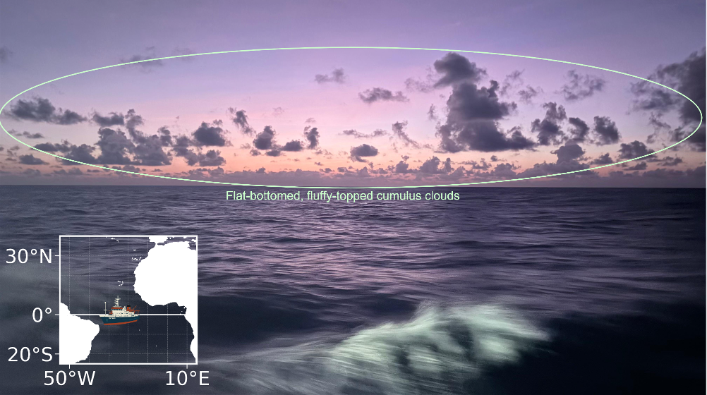
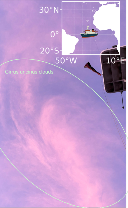
When we approached the equator, we saw many cumulus clouds with remarkably flat bases, marking the lifting condensation level where warm, moist air rising from the ocean cooled to its dew point and condensed into droplets. Similar temperature/humidity across an area leads to clouds sharing flat bases. Their uneven, towering tops reflected continued turbulence and convection above this level, revealing the active vertical mixing of the tropical atmosphere (Figure 5). As moist tropical air rises toward the cold-point tropopause, it encounters extremely low temperatures. When an air mass reaches a local temperature minimum, water vapour can freeze into very thin cirrus clouds (Figure 6).
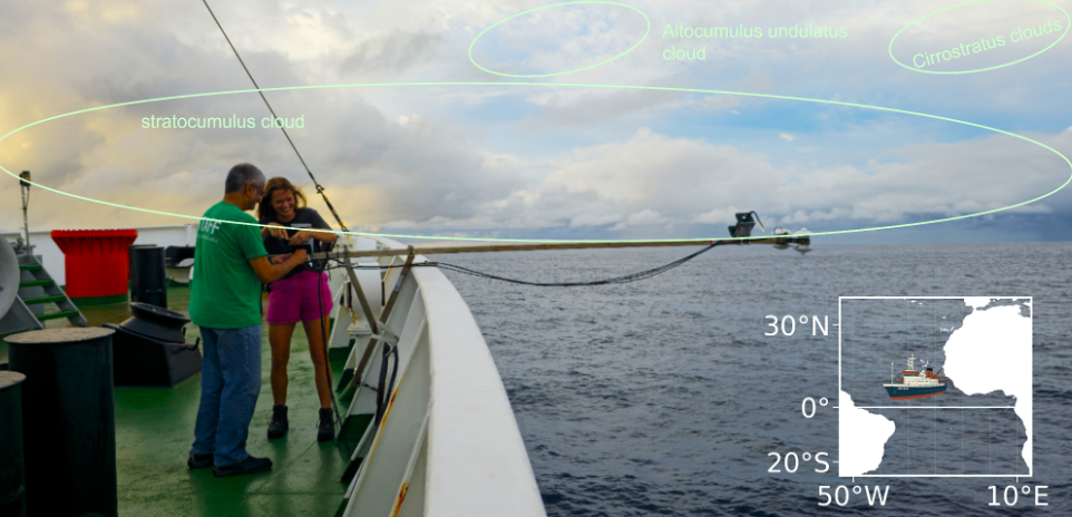
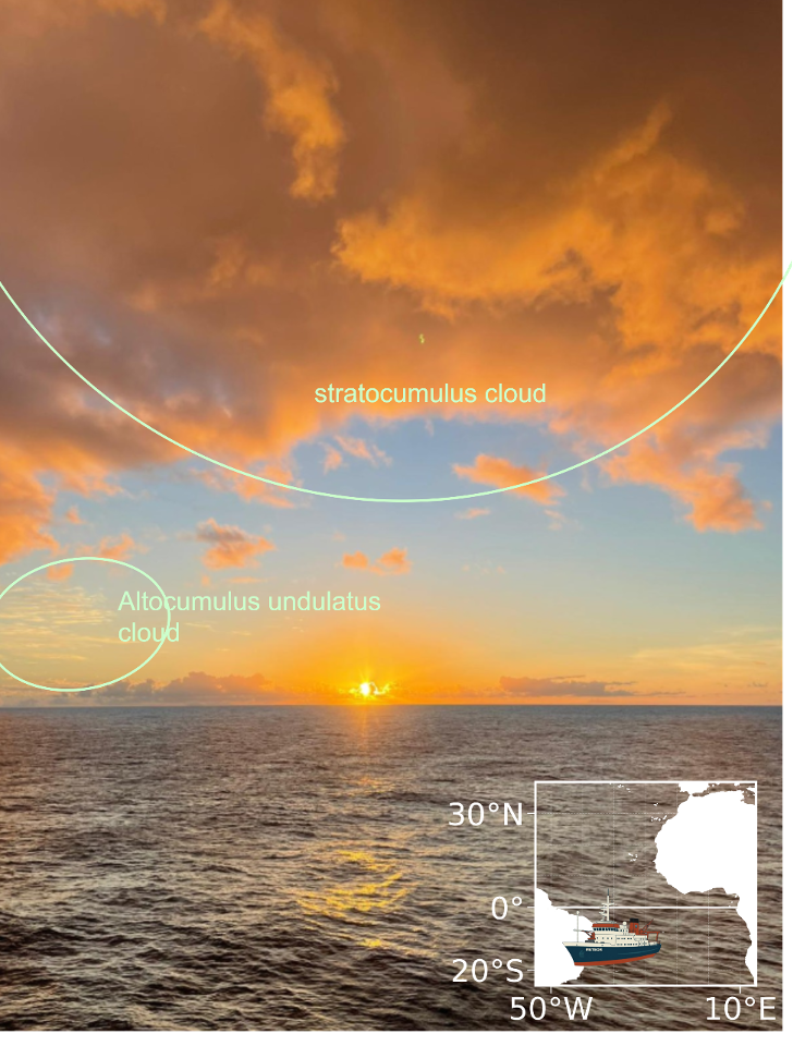
After crossing the equator, we entered the Intertropical Convergence Zone (ITCZ), a band of heavy rainfall extending across the tropical Atlantic. Cloud organization within and around the ITCZ varies markedly from day to day. Extensive low-level stratocumulus clouds can also occur in the surrounding region, acting like a blanket that reduces the amount of incoming solar radiation reaching the ocean surface (Figure 7).
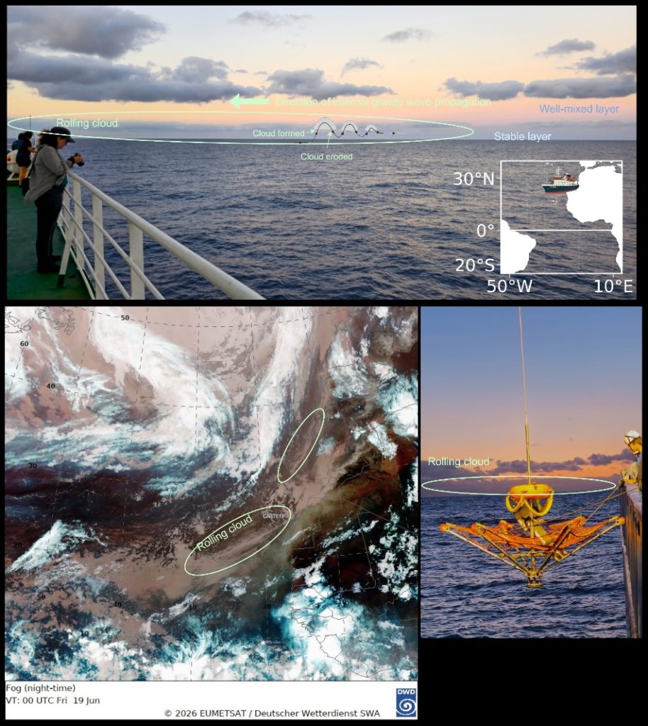
As we continued northward on our way home, we moved closer to the continent and witnessed some spectacular roll clouds, a very rare meteorological phenomenon. This type of cloud is known as “Morning Glory,” although evening land breezes can also produce roll clouds. The roll cloud is not attached to other clouds. associated with a solitary wave, a wave that has a single crest and moves without changing speed or shape.
As we were relatively close to the shoreline of West Africa, these roll clouds may have been produced by internal gravity waves propagating along a stable marine boundary layer [d]. The collision or sudden advance of a sea breeze or cold front can disturb the stable air layer near the surface, generating an atmospheric bore (a train of internal gravity waves). Such waves consist of alternating regions of upward and downward motion. Along the crest of the wave, moist air is lifted and cools to saturation, forming clouds, while behind the crest the air descends and warms, causing the cloud to evaporate. Because this cycle of ascent and descent extends along a long line of low-level convergence, cloud is continuously generated at the leading edge and dissipated at the trailing edge, maintaining a long, coherent band (Figure 8).
I think observing and thinking about clouds can be a nice hobby for enjoying the beauty of nature. Cloud processes are stochastic because nucleation and droplet collection do not occur at exactly the same time for every particle, even under the same environmental conditions [a]. Instead, freezing, condensation, and coalescence depend on chance microscopic events, so only some droplets become “lucky” and grow or freeze earlier than others. Perhaps cloud viewing could also give us good food for thought. After all, many cloud-related problems in climate modeling remain among the most beautiful mysteries in climate science.
Enjoy ~
References:
[a] Lamb D, Verlinde J. Physics and Chemistry of Clouds. Cambridge University Press; 2011.
[b] Levizzani, V., Kidd, C. (2025). Cloud Physics. In: Precipitation. Geophysics and Environmental Physics. Springer, Cham. https://doi.org/10.1007/978-3-031-97096-2_3
[c] Shang-Ping Xie. Subtropical climate: Trade winds and low clouds. In: Coupled Atmosphere-Ocean Dynamics. Elsevier; 2024. p. 139–163. doi:10.1016/B978-0-323-95490-7.00006-0.
[d] The Morning Glory and related phenomena. https://www.meteo.physik.uni-muenchen.de/~roger/AustralianProjects/TheMorningGlory/TheMorningGlory.html
By Naomi Krauzig (GEOMAR)
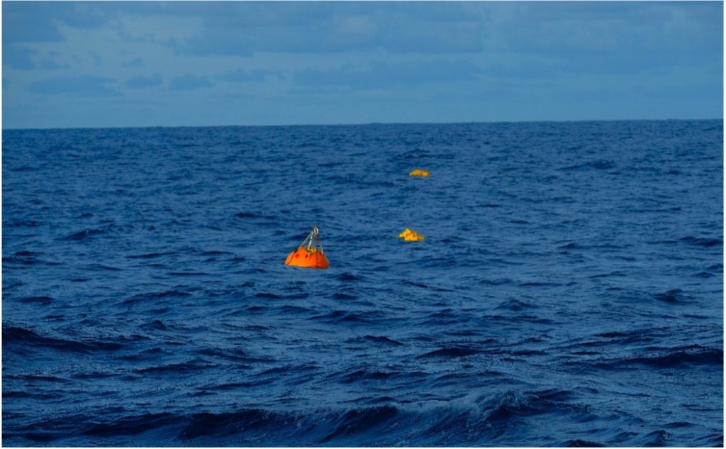
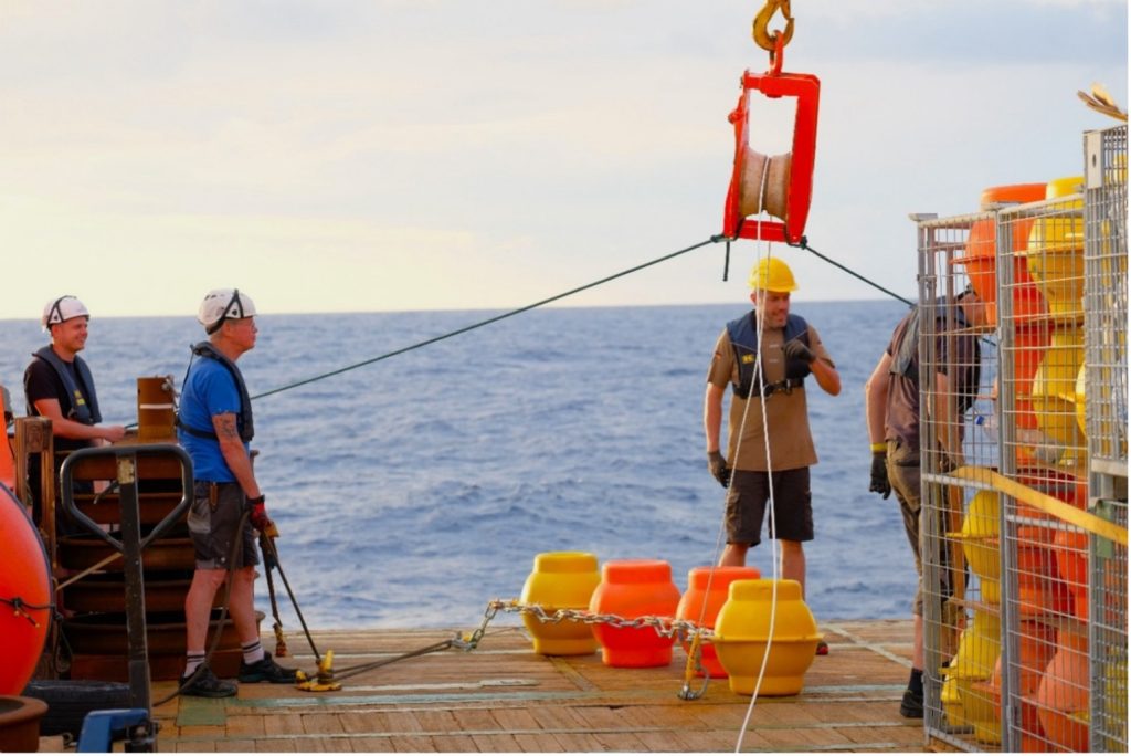
One of the most rewarding aspects of M219 has been contributing to the maintenance of the long-term GEOMAR mooring arrays that quietly monitor the tropical Atlantic year after year.
While CTD/LADCP casts and other shipboard measurements provide invaluable snapshots of the ocean, these anchored instruments provide something that cannot be obtained otherwise: continuous observations spanning minutes, days, seasons, years, and even decades. As an observational oceanographer, it is difficult not to appreciate the value of these datasets. They form the foundation for understanding ocean variability in regions that are critical for Atlantic climate variability and allow us to detect and quantify long-term changes that would otherwise remain hidden within the ocean’s natural variability.
Our first major operations took place off the Brazilian coast at 11°S, where the K1 to K4 moorings form part of a long-term observing system monitoring the western boundary current system and the Atlantic Meridional Overturning Circulation (AMOC). Within just a few days, the four deep-sea moorings were successfully recovered, assessed, serviced, and redeployed.
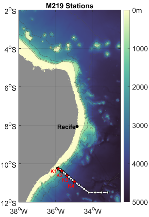
Every recovery felt a bit like opening a treasure chest. After spending a year or more beneath the ocean surface, these instruments returned carrying an invaluable record of currents, temperature, salinity, oxygen, and other key ocean properties. It was incredibly rewarding to see how well they had performed. Nearly all instruments operated successfully throughout the entire deployment period, delivering high-quality datasets with remarkably few gaps.
From Brazil, we continued north to the equator at 23°W, home to another key long-term mooring at exactly 0°N. Since 2006, this mooring has been monitoring the Equatorial Undercurrent and the deep equatorial circulation from the surface to nearly 4,000 m depth. Its successful recovery and redeployment mean that this unique 20-year time series will continue, helping us better understand how the tropical Atlantic influences climate, oxygen and nutrient transport, and marine ecosystems across the basin.
Our final mooring destination brought us to the Cape Verde Ocean Observatory (CVOO), one of the flagship long-term ocean observatories in the eastern tropical Atlantic. Here, physical, biogeochemical, and ecological observations come together to track how the ocean stores heat and carbon and how marine ecosystems respond to environmental change. Like the moorings at 11°S and the equator, the value of CVOO lies not in a single measurement, but in the continuity of the multi-decadal record.
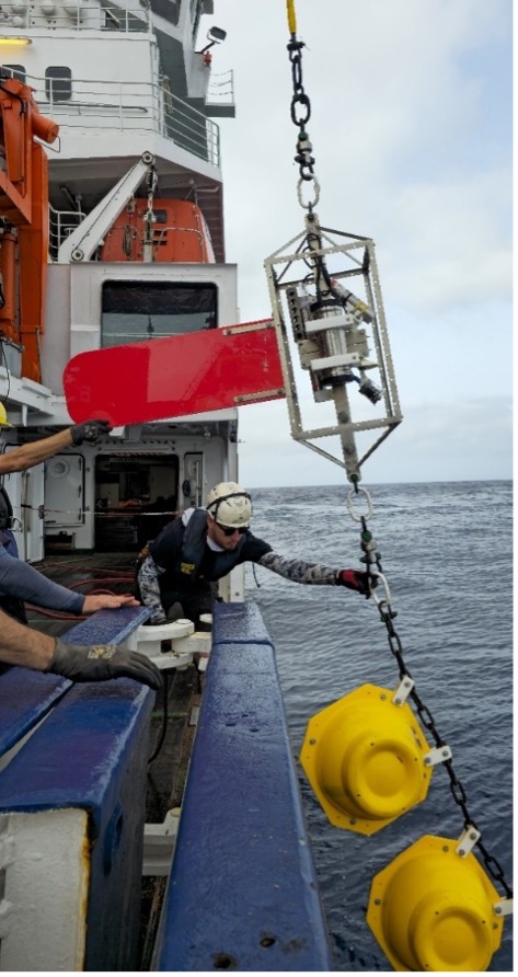
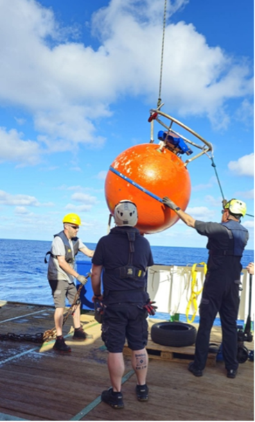
For me, one of the most memorable aspects was seeing how many people contributed to the success of the mooring operations. Careful planning laid the foundation, while having a dedicated person keeping track of every step ensured that everything ran smoothly (kudos to Anna Christina Hans, aka Tina!). On deck, crew, technicians, and scientists worked together like a well-oiled machine, stepping in where needed and solving problems on the fly.
The teamwork extended all the way back home to GEOMAR. Thanks to Rebecca Hummels’ mooring toolbox, data from several instruments could already be processed and checked while parts of the moorings were still in the water, providing an early look at the quality of the observations. On top of that, mooring experts were available around the clock to provide information, advice, and troubleshooting whenever needed. I believe the high success rate of the recoveries and redeployments is a testament to the experience, teamwork, and dedication of everyone involved.
With the major milestone of the successful mooring work behind us, another exciting operation was still ahead. Waiting in Mindelo was a brand-new surface buoy, ready to begin its own contribution to these invaluable long-term observations. Stay tuned to learn more about that deployment in a future blog post.
Keeping the Record Alive: Long-Term Ocean Observations in the Tropical Atlantic
By Joelle Habib (Laboratoire d’Océanographie Villefranche)
When you go on a scientific cruise, you always think about the instruments you’re going to deploy, the great data you’re going to acquire, or the experiments you’ll conduct. What you almost always forget is the small thing that isn’t actually small at all: food. And how are you going to eat it!
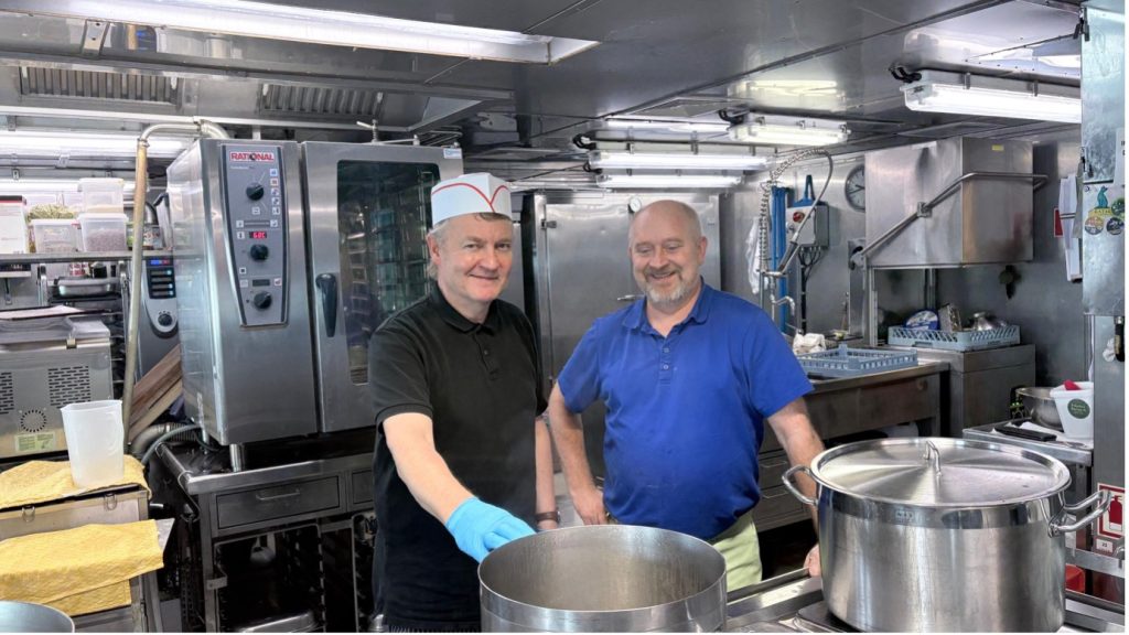
For those not familiar with scientific cruises: once you’re on board, most of your time goes to the science. You don’t really have time for food or food preparation. But there are always hidden heroes preparing your breakfast, lunch, and dinner, and, most importantly, the dessert for the dessert break. Today, instead of shedding light on the science, we’re going to talk about people, starting with the two chefs our lives basically depend on.
Rainer Götze and Peter Wernitz are the chefs of the last METEOR cruise. Rainer has been cooking on this ship for over 23 years, while Peter has been doing it for 13. Together they cook for 60 people on board, seamen and scientists alike. You’re probably wondering, like I was, how they pull it off. I had the chance to talk to them, and here are some of the ship’s secrets.
Let’s start with the planning. They don’t prepare the whole month’s menu before going on board, they plan it day by day. That said, a few dishes are practically law: fish on Tuesday and Friday, stew on Saturday (the stews are good, but it’s still my least favorite food day), and roasted meat on Sunday. Ice cream shows up for dessert on Sunday and Thursday lunches. And no matter the day, there’s always a vegetarian option on the table, nobody on board goes without something to eat.
So, all this cooking, but how many ingredients does it actually take? Let’s start with numbers. Every morning for breakfast there’s a choice of eggs (scrambled, boiled, fried…), pancakes, and more. So how many eggs are on this ship? For a one-month cruise, there are 3,000 eggs in storage, and the cooks go through around 90 of them a day. They also bake fresh bread every single day, about 3kg of flour goes into roughly 60 loaves. Coffee breaks happen all day, every day, there’s about 60kg of coffee on board. And since we’re on a German ship, and Germans do love their potatoes, there are 300kg of potatoes stored in a refrigerated, dark room so they don’t go bad.
You might be wondering why I’m talking so much about potatoes. Well, my dear reader, lunch has plenty of variety, but the one constant is potatoes. We’re on day 20 of the cruise, and I think we’ve worked through most of the varieties by now: fried, baked, soufflé, mashed, boiled and more still to come.
Another question I had was what happens if one of them gets sick. Rainer is a tough seaman who doesn’t get seasick anymore; Peter still does, occasionally. But either way, they’re always there, cooking through good conditions and bad. People generally love the food, though the chefs did tell me the one thing that never goes down well is old-school dishes like veal liver. (I can confirm.)
I think the message I’m trying to convey here is: a scientific cruise wouldn’t really be possible without Peter and Rainer. Science at sea is not only the science, but it’s also the work and effort of everyone on board. Especially the chefs!


-
Greenhouse Gases10 months ago
Guest post: Why China is still building new coal – and when it might stop
-
Climate Change10 months ago
Guest post: Why China is still building new coal – and when it might stop
-

 Greenhouse Gases2 years ago
嘉宾来稿:满足中国增长的用电需求 光伏加储能“比新建煤电更实惠”
-

 Climate Change2 years ago
嘉宾来稿:满足中国增长的用电需求 光伏加储能“比新建煤电更实惠”
-
Climate Change2 years ago
Bill Discounting Climate Change in Florida’s Energy Policy Awaits DeSantis’ Approval
-

 Renewable Energy8 months ago
Sending Progressive Philanthropist George Soros to Prison?
-

 Carbon Footprint2 years ago
US SEC’s Climate Disclosure Rules Spur Renewed Interest in Carbon Credits
-
Greenhouse Gases11 months ago
嘉宾来稿:探究火山喷发如何影响气候预测