

Human-caused emissions of aerosols – tiny, light‑scattering particles produced mainly by burning fossil fuels – have long acted as an invisible brake on global warming.
This is largely because they absorb or reflect incoming sunlight and influence the formation and brightness of clouds.
These combined effects act to lower regional and global temperatures.
Aerosols also have a substantial impact on human health, with poor outdoor air quality from particulate matter contributing to millions of premature deaths per year.
Efforts to improve air quality around the world in recent decades have reduced aerosol emissions, bringing widespread benefits for health.
However, while cutting aerosols clears the air, it also unmasks the warming caused by carbon dioxide (CO2) and other greenhouse gases (GHGs).
In this explainer, Carbon Brief unpacks the climate effects of aerosols, how their emissions have changed over time and how they could impact the pace of future warming.
Key points include:
- Clean air rules are driving a rapid decline in sulphur emissions around the world. Global sulphur dioxide (SO2) emissions have fallen by around 40% since the mid‑2000s.
- There is around half a degree of warming today that is “hidden” by aerosols. Without the cooling from sulphate and other aerosols, today’s global temperature would already be close to 2C above pre‑industrial levels, rather than the approximately 1.4C the world is currently experiencing.
- Chinese SO2 emissions have fallen by more than 70% between 2006 and 2017 as the national government has brought in a series of air-pollution measures. These declines have added around 0.06C to global warming since 2006.
- Shipping’s low‑sulphur fuel rules have added to recent warming. The International Maritime Organization’s (IMO’s) 2020 cap on marine‑fuel sulphur has already warmed the planet by an estimated 0.04C, albeit with a wide range of estimates across published studies.
- Roughly one‑quarter of the increase in global temperature over the past two decades stems from this unmasking of human-caused heat. Altogether, recent aerosol cuts may have contributed ~0.14C of the ~0.5C of warming the world has experienced since 2007.
- By unmasking warming from CO2 and other GHGs, aerosols have flipped from reducing the rate of decadal warming (as emissions increased) to increasing the rate of warming (as emissions decreased) after 2005.
- Sulphate and other aerosols are a major component of PM2.5 air pollution, which has been linked to millions of premature deaths each year.
- Most future‑emissions pathways project continued aerosol declines. Unless methane and other short-lived GHGs fall at the same time, the rate of warming could accelerate in the coming decades even if CO2 emissions plateau.
Aerosol emissions
The term “aerosols” can be a source of confusion as it often evokes images of spray cans and concerns over depletion of the ozone layer. However, aerosols are a broad category that refer to solid or liquid particles that are fine enough to remain suspended in the atmosphere for extended periods of time.
The major climate-relevant aerosols include SO2, nitrate (NO3), ammonia (NH4), mineral dust, sea spray and carbonaceous aerosols, such as black carbon and organic aerosols.
They vary in size – from nanometres to tens of micrometres – and generally have a short residence time in the lower atmosphere, lasting days to weeks before drifting back to the surface or being washed out in rain.
This means that unlike long-lived GHGs, such as CO2 or nitrous oxide (N2O), aerosols only continue to impact the climate while they are being released. If emissions stop, their climate impacts quickly dissipate.
Aerosols affect the climate by absorbing or reflecting incoming sunlight, or by influencing the formation and brightness of clouds. Most aerosols have a cooling impact because they scatter sunlight away from the Earth and back to space. However, others, including black carbon, cause warming by absorbing incoming sunlight and heating the lower atmosphere.
The figure below shows climate model output looking at the global temperature impact of each different driver of climate change (referred to as “climate forcings” or “radiative forcings”) individually. It includes GHGs, aerosols and other human-caused drivers (such as land albedo changes or tropospheric ozone), as well as natural factors (such as volcanoes and variations in solar output).
Lines above zero show forcings that have an overall warming impact, while those below zero have a cooling effect.
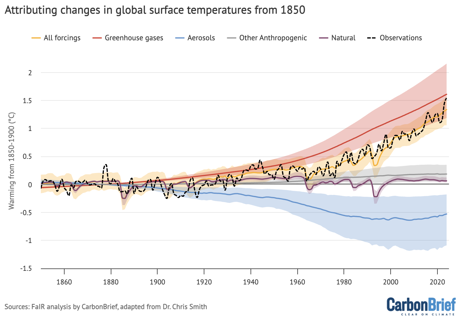
Global average surface temperature changes between 1850 and 2024 caused by each category of climate forcing. Calculated based on the FaIR climate model by comparing all-forcing model simulations to those with an individual forcing removed, following an approach developed by Dr Chris Smith. Observed surface temperatures (using the WMO average of six groups) are shown by the dashed black line.
The warming associated with GHG emissions and cooling associated with aerosol emissions are the largest factors driving the global temperature changes, particularly over the past 70 years.
In the absence of aerosol emissions, the best estimate of current warming would be approximately 0.5C higher, with the world approaching 2C rather than the 1.4C that the world is experiencing today.
Cooling from aerosols has likely masked a substantial portion of the warming that the world would otherwise have experienced.
Different aerosols and their climate effects
There are a number of different types of aerosols, whose climate impacts vary based on both the properties of the particles and the magnitude of human emissions. Of these, SO2 – often referred to as just “sulphur” – has the largest climate impact and is responsible for the bulk of aerosol masking (around -0.5C) that is occurring today.
Black carbon has a modest warming effect on the climate globally (~0.1C), but a much larger impact on Arctic temperatures where it can darken snow and ice, increasing the sunlight they absorb from the sun.
Organic carbon emissions have a modest cooling effect (around -0.1C), while emissions of ammonia and nitrate have an even-smaller cooling effect (around -0.02C). Others, such as dust and sea salt, are primarily natural and changes have had negligible effects on global temperatures.
The table below, adapted from the IPCC AR6 climate science report, provides details on the major aerosols, including their primary sources, effective radiative forcing and temperature impacts over the 1750-2019 period.
| Aerosol type | Primary sources | Effective radiative forcing in watts per metre squared (w/m2), 1750-2019 | Temperature impact, 1750-2019 |
|---|---|---|---|
| Sulphur / Sulphate (SO4) | Fossil fuel and biomass SO2 | -0.9 (-1.6 to -0.3) | Strong cooling with -0.5C (-0.1C to -0.9C) of offset warming globally. Dominant aerosol cooling component. |
| Black carbon (BC) | Incomplete combustion (diesel, coal, biomass) | 0.1 (-0.2 to 0.4) | Warming of 0.1C globally (-0.1C to 0.3C). Offsets some cooling; major regional Arctic impact. |
| Organic carbon (OC) | Biomass burning, biofuel and volatile organic compounds (VOCs) | -0.2 (-0.4 to 0.0) | Cooling of -0.1C globally (-0.2C to 0C). |
| Nitrate (NO3) and ammonia (NH3) | Nitrous oxide (NOX) from vehicles and industry and ammonia (NH3) from agriculture | -0.03 (-0.07 to 0.00) | Small global cooling effect of -0.02C (-0.05C to 0.01C). Regionally important where ammonia is abundant. |
| Dust (mineral) | Natural (deserts); some land-use change | ~0 (uncertain, ±0.1) | Small globally with an uncertain sign, but potentially larger regional effects. Anthropogenic fraction of dust forcing is small. |
| Sea salt | Ocean spray (natural) | 0 (natural baseline) | No trend or forcing attributable to human activity. |
Aerosol cooling was relatively modest until around 1950, after which SO2 emissions substantially increased worldwide, driven by a rapid increase in coal combustion and industrial activity.
The cooling effect of aerosols peaked around the year 2000 and has been declining over the past two decades. The figure below highlights the impact of aerosols on global temperature change over time.
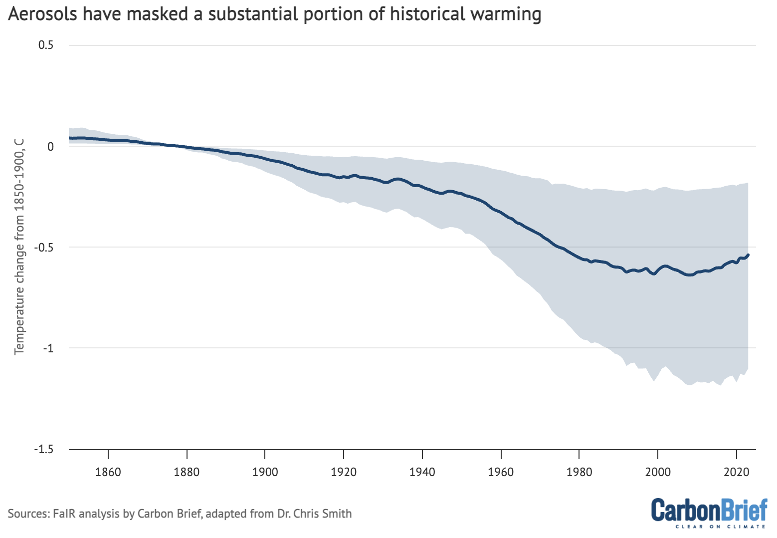
Global average surface temperature changes over 1850-2024 caused by aerosols, based on the FaIR climate model.
However, the cooling effects of aerosols remain uncertain due both to their regional nature and the complex nature of interactions between aerosols and clouds.
There is also a relationship between aerosol forcing and climate sensitivity, which is a measure of how much warming is expected from a doubling of atmospheric CO2. In general, climate models with a higher sensitivity tend to have higher aerosol cooling that counterbalances the larger GHG-driven warming. The reduction of uncertainty in aerosol cooling – particularly the effects of aerosols on cloud formation – is a major focus of scientists in their attempts to reduce the uncertainty in climate sensitivity estimates.
The climate impacts of aerosols are broadly divided into two groups, shown in the chart below. The first is a direct effect (blue line), where they scatter and absorb incoming radiation from the sun, preventing it reaching the Earth’s surface. The second is an indirect effect (dark blue line) on cloud formation, where aerosols serve as “condensation nuclei” around which clouds form.
For example, aerosols can enhance the coverage, reflectance and lifetime of low-level clouds, causing a strong cooling effect.
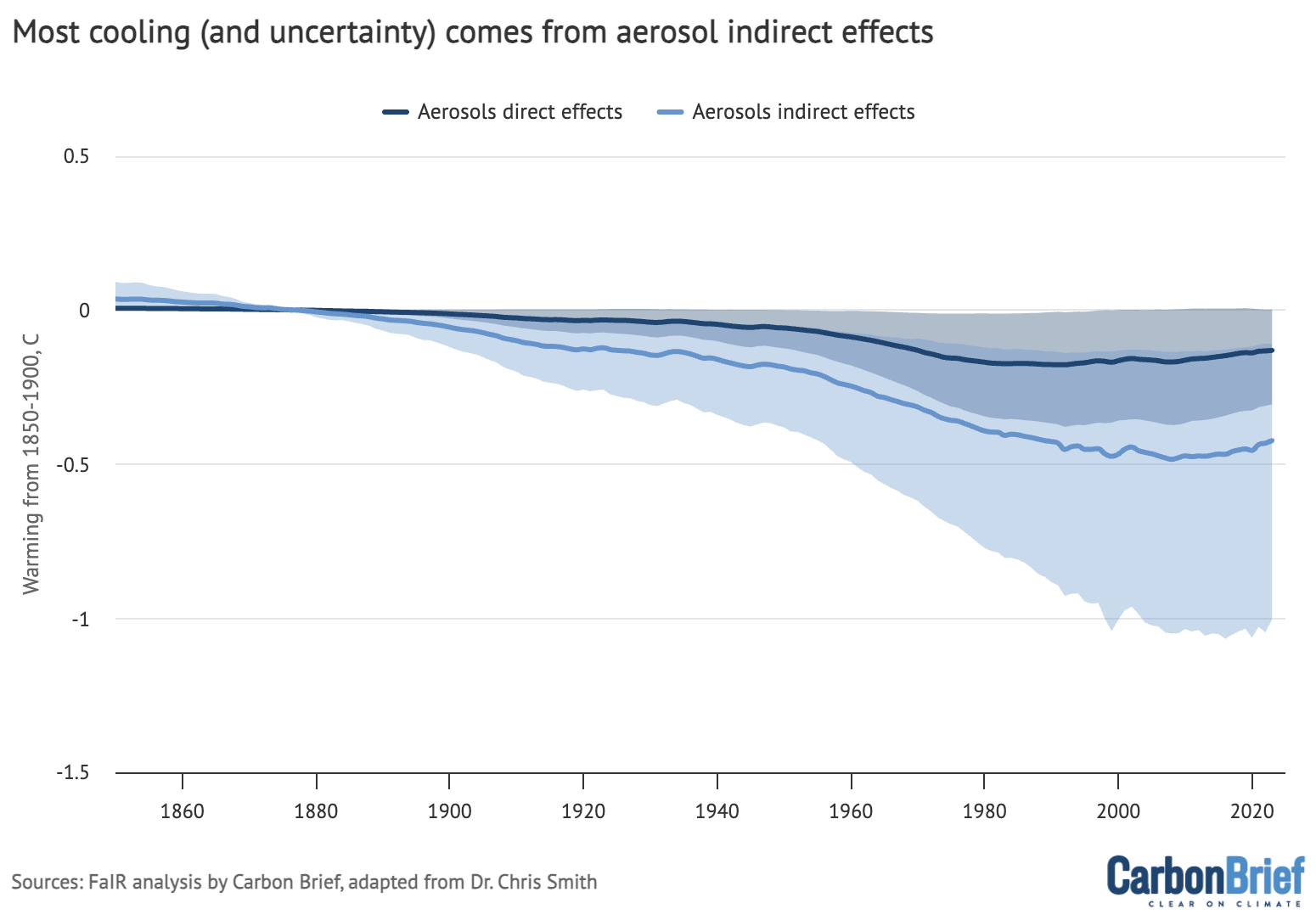
Global average surface temperature changes between 1850 and 2024 caused by direct and indirect aerosol effects, based on the FaIR climate model.
Of the two, direct aerosol effects generally have the smaller effect, with less uncertainty around their impact. They cool the planet by around -0.13C (-0.31C to 0C) today.
Indirect aerosol effects have a larger magnitude and uncertainty, with a -0.42C (-1C to -0.11) cooling impact globally today.
The recent sixth assessment report (AR6) report from the Intergovernmental Panel on Climate Change (IPCC) increased the estimated magnitude of indirect aerosol forcing, compared to the fifth assessment report (AR5). This increase was based on an improved understanding and modelling of aerosol-cloud adjustments.
While global average temperature is the focus here, it is important to note that – unlike CO2 and other GHGs – aerosols in the lower atmosphere are not “well mixed”. That is, they are not spread evenly through the atmosphere.
Rather, their short lifetime results in strong regional variation in aerosol concentrations and associated climate effects, which can have a large impact on local temperature and rainfall extremes. Regions such as east or south-east Asia, which have high sulphur emissions, have experienced larger aerosol cooling than regions with lower emissions.
The one exception is when aerosols are injected higher up in the atmosphere in the stratosphere. There, they tend to have a much longer lifetime – measured in years rather than days – and are much more well-mixed.
(Today, meaningful increases in stratospheric aerosols only occur as a result of particularly explosive eruptions of sulphur-rich volcanoes, which cool the Earth for a few years after a major eruption. However, intentionally introducing sulphate aerosols into the stratosphere has been proposed as a potential “geoengineering” strategy to temporarily mask the effects of warming. These ideas have been controversial in the scientific community.)
Aerosol emissions have a huge impact on public health. The substances are generally considered to be conventional air pollutants and are precursors of fine particulate matter air pollution (PM2.5).
Outdoor air pollution associated with sulphur and other aerosol emissions contributes to millions of premature deaths annually. As a result, much of the impetus to rapidly cut aerosols arises from public health concerns. Despite the contribution to more rapid warming, a reduction in aerosols represents a massive improvement in health and welfare for people worldwide.
Rapid declines in global sulphur emissions
Global emissions of the most climatically important aerosol – SO2 – have declined precipitously since peaking around 50 years ago.
SO2 cuts were initially driven by clean air regulations adopted by the US, UK and EU in the 1970s and 1980s in response to the growing effects of SO2 on both air pollution and acid rain.
As the figure below illustrates, SO2 emissions across the US, UK and EU have subsequently fallen from 68m tonnes per year in 1973 to just 3.3m tonnes per year today.
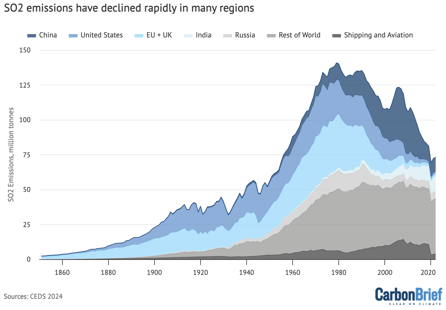
Annual SO2 emissions by country and by international shipping and aviation, 1850-2022. Data from the Community Earth atmospheric Data System (CEDS).
In the first decade of the 21st century, SO2 cuts in the UK, US and EU were counterbalanced by growing SO2 emissions in China, driven by a rapid expansion of coal use and industrial activity.
Between 2000 and 2007, global SO2 emissions saw a renewed increase, as China’s SO2 emissions reached 38m tonnes per year by 2006.
However, following an international and domestic focus on air pollution in the aftermath of the 2008 Beijing Olympics, China embarked on an ambitious programme to clean up air pollution. The nation has since cut its SO2 emissions by more than 70% to around 10m tonnes of SO2 today.
Meanwhile, SO2 emissions from global shipping recently dropped by around 65%, after the IMO instituted regulations requiring the use of low-sulphur marine fuels from 2020.
Many other countries have also broadly seen aerosol declines since 1990, although there are exceptions. For example, India’s expansion of coal generation has driven increasing SO2 emissions.
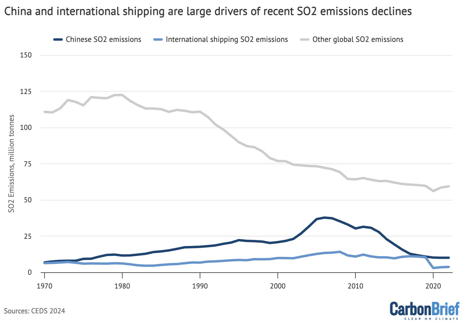
Annual SO2 emissions from China, international shipping and the rest of the world. Data from the Community Earth atmospheric Data System (CEDS).
While global SO2 emissions started decreasing in the 1980s, these declines were relatively modest until around 2008, after which they have dropped precipitously.
Global SO2 emissions today are 48% lower than they were in 1979 and 40% lower than in 2006.
It is this recent rapid decline in global SO2 emissions that has driven the reduction in overall global aerosol cooling – and a subsequent decline in the associated masking of GHG warming – discussed earlier.
Effects of low-sulphur shipping fuel
The climate effects of the IMO’s 2020 phase-out of most of the sulphur content in shipping fuel has received a lot of attention over the past two years (see Carbon Brief’s earlier coverage of the topic).
This has been explored by researchers as a potential explanation for the record levels of warming the world has experienced in recent years.
Determining the climate effects of low-sulphur shipping fuel is less straightforward than simply assessing the reduction in global SO2 emissions.
The impact of additional SO2 emissions on cloud formation diminishes as emissions increase, meaning that reductions in SO2 over areas with low background sulphate concentrations, such as the ocean, could result in a proportionately larger warming effect than in highly polluted areas, such as south Asia.
This is somewhat countered by the concentration of shipping in specific “lanes” and by natural emissions of dimethyl sulphide produced by algae that are not present on land. Assessing the radiative forcing impact of the IMO’s 2020 regulations in greater detail requires the use of sophisticated climate models that can simulate these regional effects.
Carbon Brief conducted a survey of the literature on the climate impacts of the 2020 low-sulphur marine fuel regulations. Of eight studies published in peer-reviewed journals over the past two years, shown in the chart below, most determined a radiative forcing change of around 0.11 to 0.14 watts per meter squared (w/m2).
One estimate from Skeie et al. (2024) was a bit lower at around 0.08 w/m2 and another from Hansen et al. (2025) was substantially higher than all the others at 0.5 w/m2.
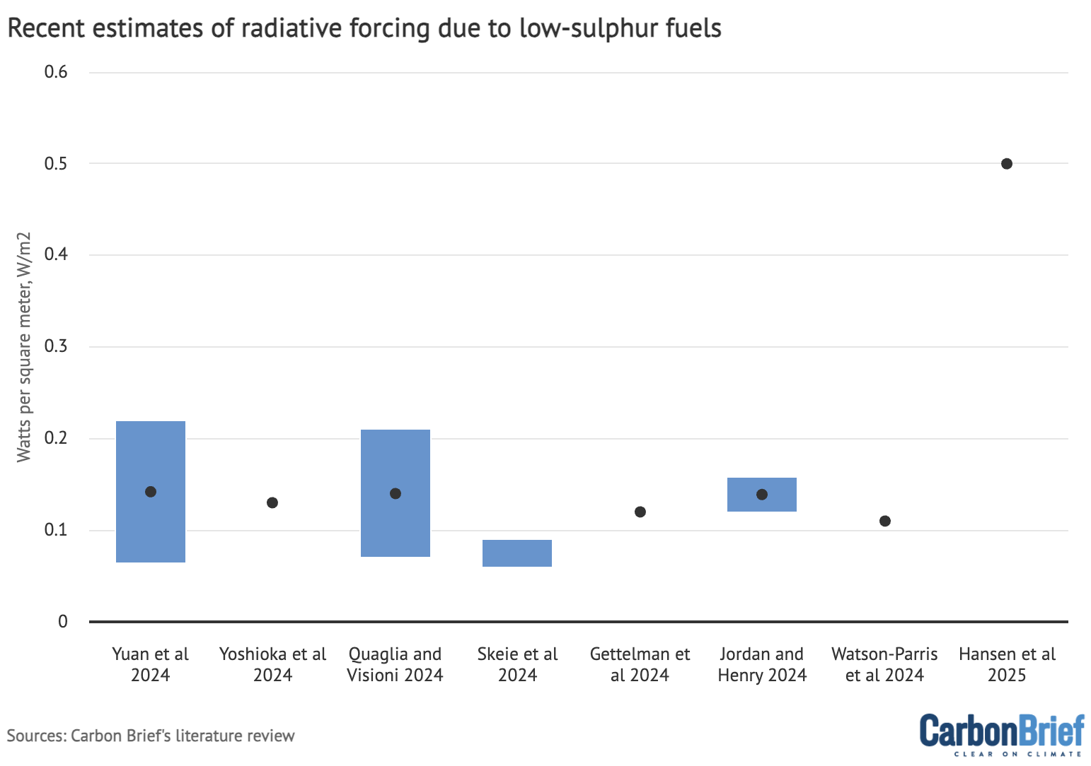
Estimates of global average radiative forcing changes from the IMO 2020 regulations published in the last two years. See the Methodology section for links to individual studies.
To account for these differing studies, Carbon Brief used the FaIR climate model emulator to simulate the effects of the radiative forcing estimated in each study on global average surface temperatures between 2020 and 2030. This includes 841 different simulations for each study to account for uncertainties in the climate response to aerosol forcing. (See: Methodology for further details.)
These estimates were then all combined to provide a central estimate (50th percentile) that gives each study equal weight, as well as a 5th to 95th percentile range across all the simulations for each different forcing estimate, as shown in the figure below.
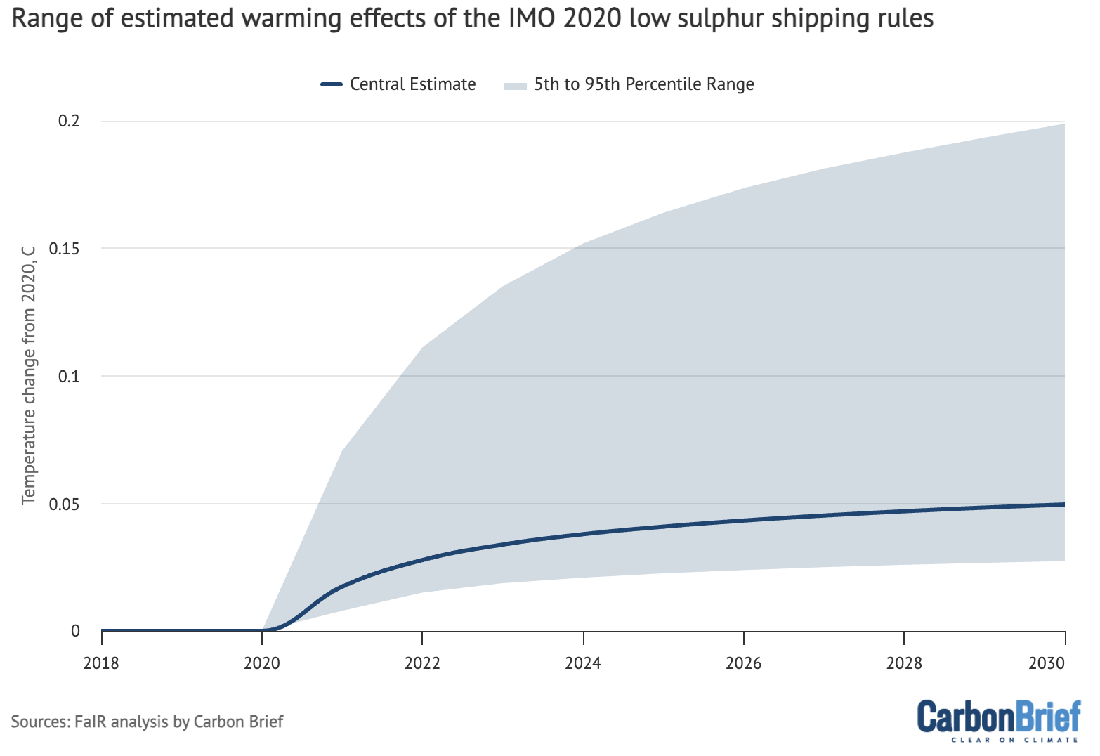
Range (5th to 95th percentile) and central estimate (50th percentile) of simulated global average surface temperature responses to the IMO 2020 regulations across the radiative forcing estimates in the literature. Analysis by Carbon Brief using the FaIR model.
Overall, this approach provides a best estimate of 0.04C (0.02C to 0.16C) additional warming from the IMO’s 2020 regulations as of 2025, increasing to 0.05C (0.03C to 0.2C) by 2030.
These large uncertainty ranges are due to the inclusion of the Hansen et al. (2025) estimate, which represents something of an outlier relative to other published studies. Note that the warming of the climate system associated with the IMO 2020 regulations increases over time in the plot due to the ocean’s slow rate of warming buffering the climate response to forcing changes.
Declines in Chinese SO2 are unmasking warming
China’s reduction of SO2 emissions by more than 70% since 2007 represents a remarkable public health success story. It is estimated to have prevented hundreds of thousands of premature deaths from air pollution annually.
These rapid emissions cuts by China represent more than half the reduction in global SO2 emissions since 2007. They have been a major contributor to global temperature increases over the past two decades.
To determine the impact of Chinese SO2 reductions on global average surface temperatures, Carbon Brief used Chinese SO2 emissions data from the Community Emissions Data System (CEDS) combined with the FaIR climate model emulator.
The figure below shows the central estimate and 5th to 95th percentile across 841 different FaIR model simulations to account for uncertainties in the climate response to SO2 emissions.
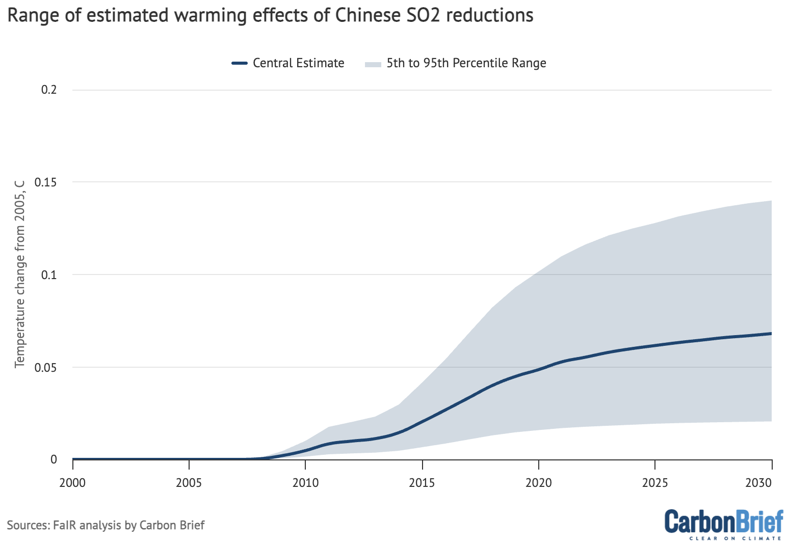
Range (5th to 95th percentile) and median (50th percentile) of simulated global mean surface temperature responses to declines in Chinese SO2 emissions. Analysis by Carbon Brief using the FaIR model.
The figure above shows that Chinese SO2 declines were likely responsible for a global temperature increase of around 0.06C (0.02C to 0.13C) between 2007 and 2025, increasing to 0.7C (0.02C to 0.14C) by 2030.
Much of this increase occurred between 2007 and 2020, with a more modest contribution of Chinese aerosol changes to warming in recent years.
These results are nearly identical to those found in a study currently undergoing peer review by Dr Bjørn Samset and colleagues at CICERO, which finds a best estimate of 0.07C (0.02C to 0.12C) using a large set of simulations from eight different Earth system models.
This suggests that Chinese SO2 reductions are responsible for approximately 12% of the around 0.5C warming the world experienced between 2007 and 2024.
What aerosol cuts mean for current and future warming
It is clear that rapid reductions in global SO2 emissions have had a major impact on the global climate.
The combination of declines in emissions since 2007 in China and the rest of the world, along with declines in SO2 from shipping after 2020, have collectively unmasked a substantial amount of warming driven by GHGs.
While the reduction in SO2 emissions in other countries has been proportionately smaller than that seen in China, collectively it adds up to 0.03C (0.01C to 0.07C) of warming in 2025.
The figure below provides a best-estimate of all three factors: declines in SO2 emissions in shipping, China and the rest of the world.
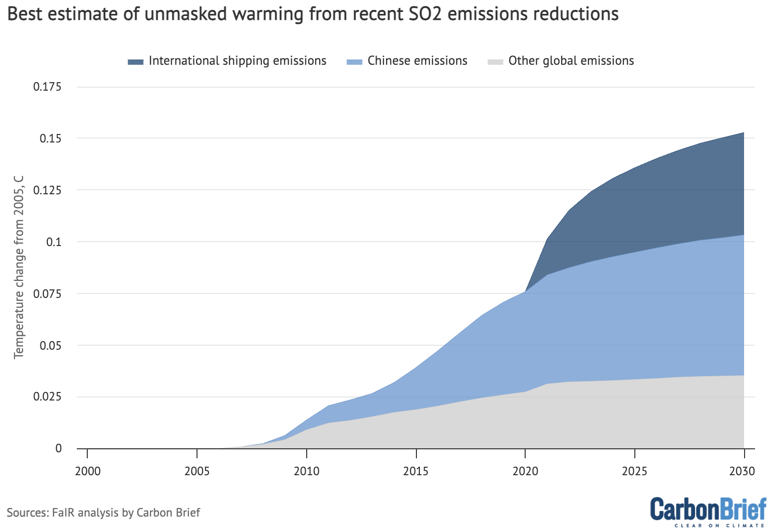
Combined central (50th percentile) estimates of modeled global average surface temperature changes from IMO 2020, Chinese SO2 and rest-of-world SO2 declines between 2005 and 2030. Analysis by Carbon Brief using the FaIR model.
Taken together, these declines in SO2 emissions may represent around 0.14C additional warming today, or more than a quarter of the approximately 0.5C warming the world has experienced between 2007 and 2024.
However, the uncertainty in the climate response to changes in aerosol emissions remains large, particularly for changes in shipping emissions, so it is hard to rule out either a much smaller or much larger effect.
These results are in line with other recent analyses showing that changes in aerosol emissions are contributing to an increase in the rate of human-caused global warming in recent years.
The figure below uses a similar FaIR-based climate modeling approach to assess how different factors contributing to human-caused warming have changed over time.

Drivers of decadal warming rates between 1970-1979 and 2015-2024, excluding natural factors like volcanoes and solar cycle variation. From an analysis using the FaIR model at The Climate Brink, adapted from earlier work by Dr Chris Smith.
This shows that the rate of human-caused warming remained relatively flat at around 0.18C per decade from 1980 to 2005, before accelerating to around 0.27C over the past decade.
The primary driver of this recent acceleration in warming has been declining aerosol emissions.
Aerosols have flipped from reducing the rate of decadal warming (as emissions increased) to increasing the rate of warming (as emissions decreased) after 2005 by unmasking warming from CO2 and other GHGs.
The rate of warming from CO2 has increased over time as emissions have increased, though it has plateaued over the past decade as increases in global emissions have slowed.
However, the rate of warming from all GHG emissions – CO2, methane and others – has been relatively consistent since 1970. This is primarily due to the declining contribution of other GHGs to additional warming, likely associated with the phaseout of halocarbons after the Montreal Protocol.
Future declines in aerosols are expected in most of the Shared Socioeconomic Pathways (SSPs) used to simulate potential levels of future warming for the IPCC AR6 report, as shown in the figure below.
Modelled future SO2 emissions are generally dependent on broader mitigation trends – worlds with less fossil-fuel use result in less sulphur emissions – but are also highly variable across different models.
Observed SO2 emissions (black line) are broadly at the same level as (though slightly below) the SSP2-4.5 scenario (yellow line), which is the pathway that most closely matches current climate policies.
Observed SO2 emissions are also similar to those in the very-high emissions SSP5-8.5 scenario (lower grey line), while being higher than emissions in the most ambitious mitigation scenario (SSP1-1.9, green line) and below those in the SSP1-2.6 scenario (navy blue line).
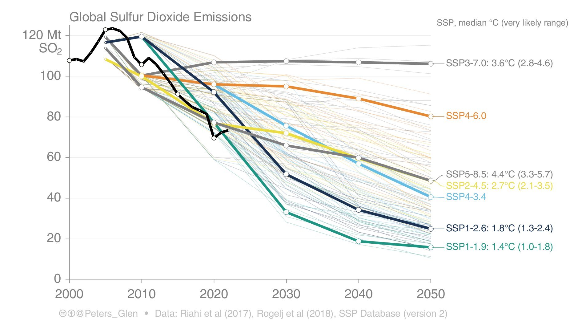
Given differences across modeling groups, it is hard to infer too much about which SSP scenario is most in line with real-world SO2 emissions. However, it is worth noting that the current SSPs do not include a scenario where SO2 emissions continue to rapidly decline while emissions of CO2 and other GHGs increase.
Interestingly, the best-estimate cooling effect from sulphur dioxide is more or less counterbalanced by the warming effect of methane emissions today. As a result, scenarios where all GHG emissions are brought to zero do not result in sustained additional warming due to unmasking from declining aerosols.
However, if CO2 emissions alone were reduced to zero, while non-CO2 emissions were held constant, cutting global aerosol emissions to zero would result in between 0.2C and 1.2C of additional warming.
This means that aerosol emissions represent something of a wildcard for future warming over the 21st century. Continued rapid reductions in SO2 emissions will contribute to an acceleration in the rate of global warming in the coming years.
Methodology
Carbon Brief used the FaIR climate model to determine the effects of aerosol emissions on the climate, building on the work of Dr Chris Smith. Runs were done using the constrained ensemble approach using “fair-calibrate v1.4.”1 to be consistent with the IPCC AR6 parameter range. More details on the constrained ensemble approach can be found in Smith et al. (2024).
Figures showing the global mean surface temperature impact of different climate forcings in isolation were performed by calculating the difference between all-forcing runs and runs where a single forcing (e.g. from GHG emissions) was removed, following the approach used to generate Figure 7.8 in the IPCC AR6 climate science report.
IMO 2020 forcing estimates were taken from the following studies published in the peer-reviewed literature over the past two years:
- Yuan et al. (2024)
- Yoshika et al. (2024)
- Quaglia and Visioni (2024)
- Skeie et al. (2024)
- Gettelman et al. (2024)
- Jordan and Henry (2024)
- Watson-Parris et al. (2024)
- Hansen et al. (2025)
IMO 2020 global average surface temperature changes were calculated by running 841 different FaIR simulations for each of the different forcing estimates identified in the literature, which is the default setting for the FaiR constrained ensemble to provide a range of results consistent with the IPCC AR6 parameter range.
This produced 6,728 total simulations, from which a central (50th percentile) estimate and uncertainty range (5th to 95th percentile) were calculated.
These results were further validated by comparing them to the Earth system model-based estimates in individual studies where near-term global average surface temperature change estimates were provided (Yoshika et al. (2024); Quaglia and Visioni (2024); Gettelman et al. (2024); Jordan and Henry (2024); Watson-Parris et al. (2024); and Hansen et al. (2025).
The results of each of these studies were within the range of FaIR based estimates for the respective study’s radiative forcing – and generally quite close to FaIR’s median estimate for that study, as shown in the table below.
| Study | Carbon Brief’s Estimate (2025) | Published Estimate |
|---|---|---|
| Yoshika et al., 2024 | 0.041C (0.032C to 0.053C) | 0.04C |
| Quaglia and Visioni, 2024 | 0.044C (0.034C to 0.057C) | 0.08C (0.05C to 0.11C) |
| Gettelman et al., 2024 | 0.038C (0.029C to 0.049C) | 0.04C |
| Jordan and Henry 2024 | 0.044C (0.034C to 0.057C) | 0.046C (0.036C to 0.056C) |
| Watson-Parris et al., 2024 | 0.035C (0.027C to 0.045C) | 0.03C (-0.09C, 0.19C) |
| Hansen et al., 2025 | 0.157C (0.123C to 0.205C) | 0.2C |
It is worth noting that the uncertainties associated with converting SO2 forcing estimates to warming outcomes are generally much smaller than converting SO2 emissions into warming outcomes.
The effect of Chinese SO2 reductions were based on a comparison of two scenarios. The first is where Chinese SO2 emissions remained constant at their peak (2007) levels and did not decline. The second is where Chinese emissions followed observational estimates from CEDS between 2005 and 2022 and then remained constant at 2022 levels thereafter (which represents a conservative assumption that likely underestimates future effects of SO2 emissions declines on global temperatures given the strong downward trend). Global average surface temperature changes were calculated by running 841 different FaIR simulations in emissions mode for two scenarios and analysing the difference between the two.
The resulting estimate of 0.06C (0.02C to 0.13C) warming by 2025 was validated by comparing it to the Samset et al. (2025) preprint, which finds a nearly identical best estimate of 0.07C (0.02C to 0.12C) using a large set of simulations from eight different Earth system models.
The effects of the rest of the world’s SO2 declines were estimated using the same approach used for Chinese SO2 emissions, using CEDS emissions data. International shipping and aviation aerosols were excluded from the rest of the world estimate as to not double count IMO 2020 effects.




The post Explainer: How human-caused aerosols are ‘masking’ global warming appeared first on Carbon Brief.
Explainer: How human-caused aerosols are ‘masking’ global warming

Cleaner cooking projects in the UN carbon market will have to set aside a share of their credits to insure against the risk that the trees they save are lost to fire, drought or logging, after the market’s regulator rejected calls to exempt the sector.
The requirement is part of a new rulebook that the Paris Agreement carbon market regulator – the Article 6.4 Supervisory Body –