
Recently, you may have heard about something called “El Niño.” But what exactly is El Niño and its sibling “La Niña”? Why do these terms seem to emerge from the depths of the scientific community and drop into popular vocabulary every few years? And how are they connected to extreme weather and our ocean?
What Are El Niño and La Niña?
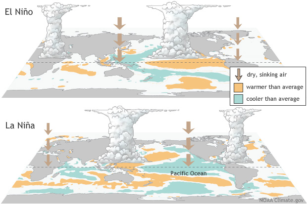
El Niño and La Niña are part of a natural climate pattern in the tropical Pacific called the El Niño-Southern Oscillation, or ENSO. These two phases are different sides of the same coin, creating equally extreme shifts in temperature and air pressure.
El Niño occurs when surface water in the equatorial Pacific becomes warmer than average and easterly winds weaken. La Niña is the opposite: cooler-than-normal sea surface temperatures and stronger easterly winds. ENSO cycles can last up to seven years. El Niño and La Niña significantly impact weather patterns in all corners of the globe, often leading to more extreme weather, storm frequency and intensity.
A strong El Niño can cause flooding in some regions and drought, heat waves and wildfires in others. It often causes crop losses, coral bleaching and marine die-offs due to unusually warm ocean temperatures. El Niño tends to suppress Atlantic hurricane activity, though it increases the risk of heavy precipitation and harm to fisheries elsewhere. In the Northern Hemisphere, El Niño typically builds between March and June, peaks in December, and weakens by February.
La Niña, by contrast, often fuels an active Atlantic hurricane season and increases tornado frequency across the southern United States. Like El Niño, it builds in spring and peaks around December.
Get Ocean Updates in Your Inbox
Sign up with your email and never miss an update.
Predicting ENSO
In 1923, the physicist Sir Gilbert Walker discovered the “Southern Oscillation,” or large-scale changes in sea level pressure across the tropical Pacific. However, it wasn’t until the late 1960s that the metorologist Jacob Bjerknes found that the changes in the ocean and the atmosphere were connected, and the hybrid term “ENSO” was born. In 1974, researchers at Oregon State University attempted to predict ENSO for the first time.
Modeling has greatly advanced since the early days. Today, scientists at the National Oceanic and Atmospheric Administration (NOAA) issue regular predictions about ENSO, which are now more accurate than ever.
NOAA gives a one-in-four chance that an El Niño could reach “very strong” intensity later in 2026, qualifying it as a “super El Niño.” This threshold has been crossed only a handful of times in recorded history, each triggering droughts, floods and record temperatures across multiple continents. NOAA’s data and models deliver life-saving early warning forecasts, like that of the predicted super El Niño, which allow communities to better prepare for and respond to extreme weather events.
Take Action
Every American, regardless of where they live, depends on NOAA’s scientists and professionals, whose work spans from the ocean floor to the far reaches of space. Unfortunately, NOAA is under threat. The Trump administration has proposed billions of dollars in cuts to the agency, which could weaken weather forecasting, disrupt fisheries management and stall critical ocean research, putting American lives and global scientific leadership at risk.
Ocean Conservancy is committed to working with NOAA to keep the public informed on climate and ocean science. We all benefit from a healthier ocean, and investing in research is the most effective way to restore ocean health and reduce the impact of severe weather events caused by El Niño and La Niña. Our ocean is not partisan, and protecting it requires all hands on deck and all sides of the aisle. Now, it’s more important than ever to demand that members of Congress prioritize our ocean. Add your name now.
The post Do You Know the Difference Between El Niño and La Niña? appeared first on Ocean Conservancy.
Ocean Acidification
Ribbegople, Rippenqualle or Comb Jelly: Whatever You Call Mnemiopsis leidyi, You Should Be Concerned
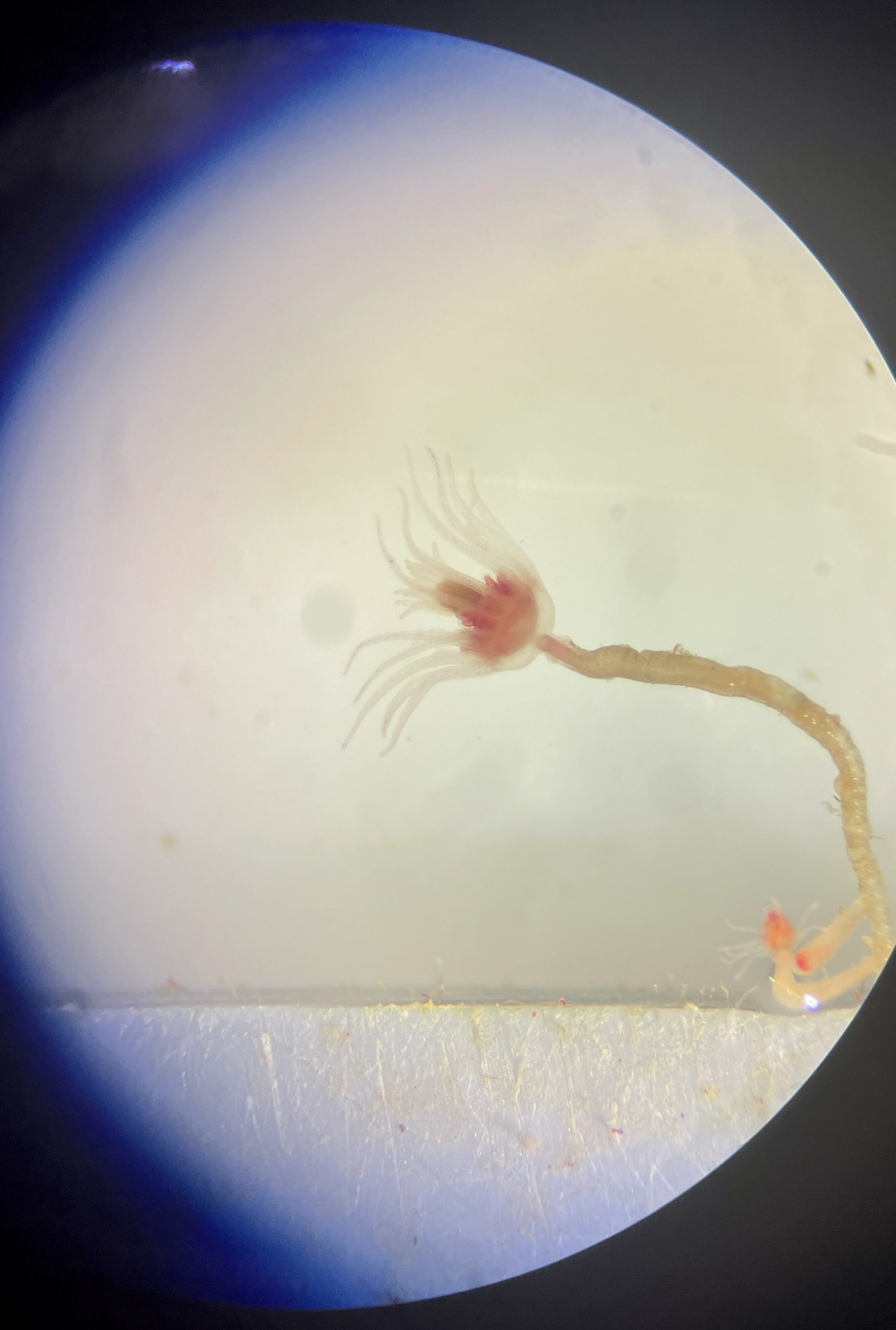
In early July at Kerteminde, most of the individuals I observed were longer than 10 cm, including one close to 15 cm. Their size, and their timing, deserve immediate attention.
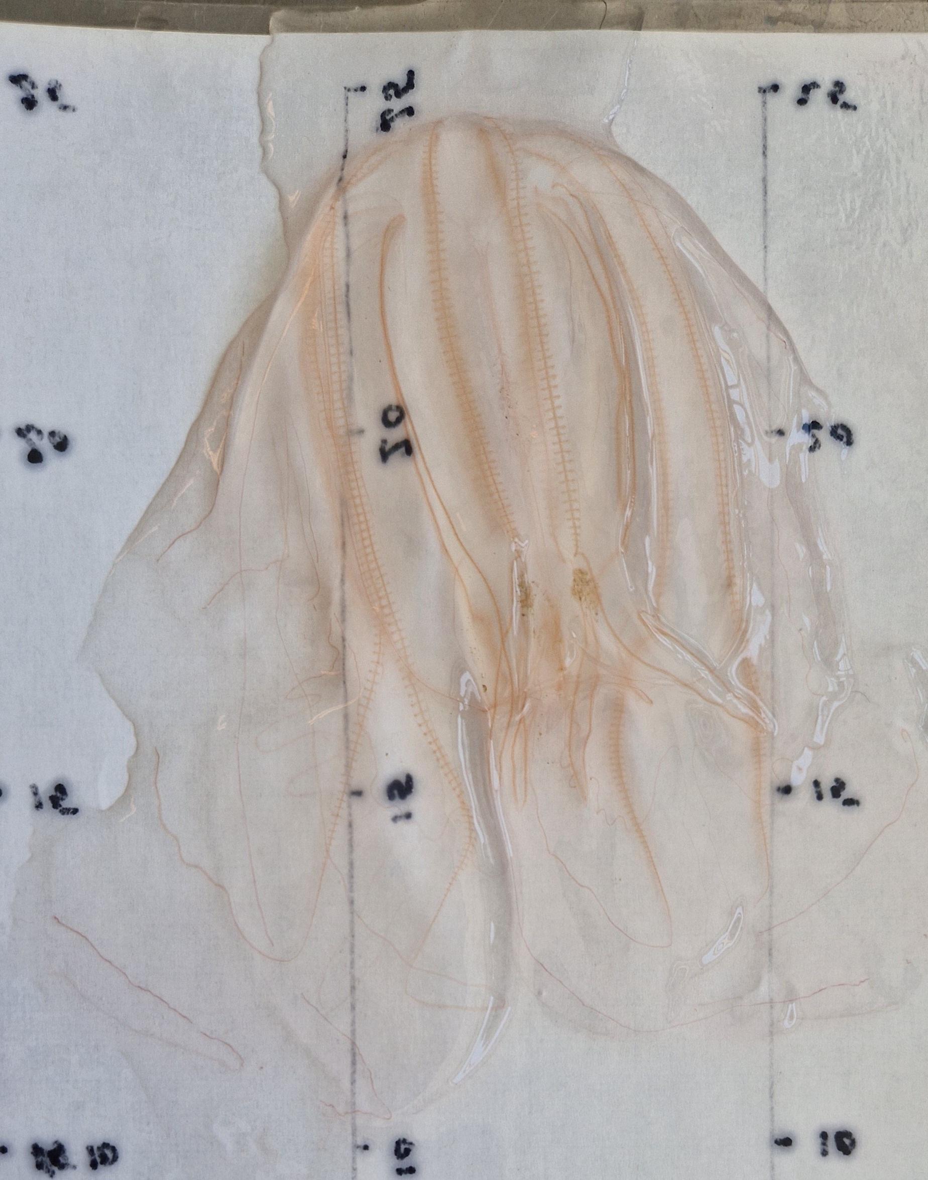
 One out of many large speciments I got from Kerteminde (Javidpour, July 2026)
It does not matter whether you call it ribbegople in Danish, Rippenqualle in German or comb jelly in English. The species is the same: Mnemiopsis leidyi. And what I have observed in Kerteminde this summer should concern us. During our current summer field course at the Marine Research Centre, I have repeatedly seen unusually large individuals of M. leidyi around the pier. Most of the animals I observed were longer than 10 cm, even bigger than the one I photographed.
Yes, yes, a pier observation is not a formal population survey….I know. We still need systematic sampling to determine the abundance, distribution and size structure of the population. Nevertheless, the observation is striking because both the size of the animals and the timing of their appearance are unusual, said by someone who is studying this species for the last 20 years.
This is happening earlier than expected
In previous years, the maximum population size of M. leidyi generally occurred several weeks later, mainly during August and early September. Our previous research, including work based on daily sampling, showed a clear seasonal development of the population. The timing varies among years and is influenced by environmental conditions, including winter temperature. Temperature is particularly important because it strongly affects the metabolism of M. leidyi. At warmer temperatures, individuals use their carbon reserves much faster and therefore require more food to maintain themselves and grow. This year, however, the pattern appears to be different. We are seeing very large individuals already in early July. We do not yet know whether this is a local aggregation, an unusually early bloom, transport from another area, particularly favourable feeding conditions or a combination of these factors. But it is a signal that deserves attention.
What does it take to grow by one centimetre?
It is tempting to ask how much energy an individual needs to add one centimetre to its body. The answer is not straightforward because one centimetre of length is not a fixed amount of biomass. Growing from 5 to 6 cm is not the same as growing from 14 to 15 cm…OK? However, we can make a rough carbon-budget calculation using a published relationship between the length and body-carbon content of M. leidyi:
Body carbon in milligrams = 0.0017 × body length in millimetres²·⁰¹³⁸
According to this relationship, an individual measuring 10 cm contains approximately 18.1 mg of carbon. At 11 cm, it contains about 21.9 mg. Adding this single centimetre therefore represents an increase of approximately 3.8 mg of body carbon. If we assume that the animal assimilates approximately 40% of the carbon it consumes, it would need to ingest at least ~10 mg of prey carbon to produce this additional tissue. Using an approximate value of 1 micrograms of carbon for a small copepod, this would correspond to more than 10,000 copepods.
For an already large individual growing from 14 to 15 cm, the estimated increase is approximately 5.3 mg of body carbon. At the same assimilation efficiency, that would require at least 13.3 mg of prey carbon: the equivalent of roughly 15,000 small copepods.
These calculations are only rough, conservative estimates. They are not complete energy budgets. They do not include the food needed for respiration, movement, reproduction, mucus production, excretion or unsuccessful feeding. The real prey requirement would therefore be considerably higher. The important point is that an individual measuring 15 cm represents a substantial transfer of material from the surrounding planktonic food web into gelatinous biomass. One additional centimetre is not “just” one centimetre.
Our students are tracing the food web
The timing of these observations coincides with our summer field course. The students are now collecting M. leidyi, fish, other gelatinous organisms and potential prey for stable-isotope analysis. By comparing carbon and nitrogen isotope values, we hope to obtain a rough picture of the relationships within the local food web. Carbon isotopes can help us trace the original sources of the material entering the food web, while nitrogen isotopes can provide information about relative trophic position.
This will not give us a direct photograph of one organism eating another. Stable-isotope values represent assimilated food over time, and their interpretation depends on appropriate baselines and turnover rates. Nevertheless, combined with information about size, abundance, prey availability and experimental feeding, they can help us understand where M. leidyi is obtaining its biomass and which organisms may be affected. …In simple terms, we are trying to determine who might be eating whom, and where this unusually large population fits into the food web.
Competition with fish is only part of the problem
The concern is not limited to competition for zooplankton. Mnemiopsis leidyi consumes copepods and other small planktonic animals that are also important food for pelagic fish. When the ctenophores are abundant, they can therefore compete directly with fish for prey. Our experiments have also demonstrated that M. leidyi can potentially feed directly on the early life stages of fish. In the study by my previous PhD student, the ctenophores captured and digested Baltic herring yolk-sac larvae. Predation was related to ctenophore size and was not simply eliminated when alternative copepod prey were available. This means that M. leidyi may/can affect fish populations in two ways: by consuming the food needed by fish and by consuming fish eggs or larvae directly.
A recent study by Lucila Sobrero and colleagues in Argentina, within the native range of M. leidyi, found a similar pattern. Their experiments showed size-dependent predation on fish eggs and larvae. Larger ctenophores consumed more eggs. Some eggs were later regurgitated, but many were no longer viable, while fish larvae were retained and digested. These findings are particularly relevant to what we are observing in Kerteminde. The size of an individual is not merely an interesting measurement. It can influence what that individual is capable of capturing and how strongly it affects the surrounding ecosystem. A population consisting of fewer but much larger individuals may still exert substantial pressure on zooplankton, fish eggs and fish larvae.
We need to investigate use, not only control
For several years, I have tried to obtain funding to investigate innovative approaches to this invasive species.
Once M. leidyi is well established, we may not be able to control its regional spread or completely prevent its blooms. But that does not mean that we have no options. We should investigate whether at least part of this recurring biomass can be collected and converted into something useful.
This is not a proposal for a miracle solution. Any utilisation strategy would have to be tested carefully. It must not encourage the further spread of the species, create damaging bycatch or provide an economic incentive to maintain an invasive population. We also need to understand the environmental costs of collection, transport and processing.
But these are exactly the questions that research funding should allow us to answer.
So far, my attempts to secure support for this work have been unsuccessful. Funding agencies do not seem to sense the urgency of studying approaches whose benefits may not be immediate or easily visible. and EPAs do not have any resource to invest in this part. The contrast with events on land is striking. This week, the oak processionary moth, the so-called “larva from hell”, has attracted considerable attention in Odense. Its microscopic hairs can cause rashes and allergic reactions, residents have reported serious discomfort, and a kindergarten has reportedly had to close temporarily. Those concerns are real and deserve a response.
But the case also illustrates how differently we react to environmental threats.
When the impact appears visibly on human skin, the urgency is immediately understood. When ecological damage develops below the surface of the sea, in the form of disappearing zooplankton, altered food webs, consumed fish eggs or reduced larval survival, it is much easier to overlook.
Marine ecosystem changes are often gradual, underwater and largely invisible to the public. By the time their consequences become obvious, the opportunity for early and relatively inexpensive action may already have passed.
Concern does not mean panic
One photograph and a series of observations from one pier do not prove that an ecological crisis is underway. I am not suggesting that they do. But science should not have to wait for undeniable damage before investigation becomes urgent.
The unusually large M. leidyi appearing in Kerteminde this July give us an opportunity to act early. We need systematic monitoring of their abundance and size distribution. We need to measure the available prey field. We need to determine their trophic position and investigate possible consequences for fish recruitment. And we need to explore whether biomass that we may be unable to prevent could be collected and used responsibly.
Whatever language we use and whatever name we give it, the message is the same:
We should measure early, investigate early and support innovative solutions while the warning is still only a warning, not after it has become a crisis.
Relevant publications
Javidpour, J. et al. (2009). “Seasonal changes and population dynamics of the ctenophore Mnemiopsis leidyi after its first year of invasion in the Kiel Fjord, Western Baltic Sea.” Biological Invasions.
Javidpour, J. et al. (2020). “Cannibalism makes invasive comb jelly, Mnemiopsis leidyi, resilient to unfavourable conditions.” Communications Biology.
Stoltenberg, I. et al. (2024). “Predation on Baltic Sea yolk-sac herring larvae (Clupea harengus) by the invasive ctenophore Mnemiopsis leidyi.” Fisheries Research.
Sobrero, L. et al. (2025). “Predatory impact on ichthyoplankton by Mnemiopsis leidyi is size-dependent: an experimental approach.” Marine Ecology Progress Series.
Ribbegople, Rippenqualle or Comb Jelly: Whatever You Call Mnemiopsis leidyi, You Should Be Concerned
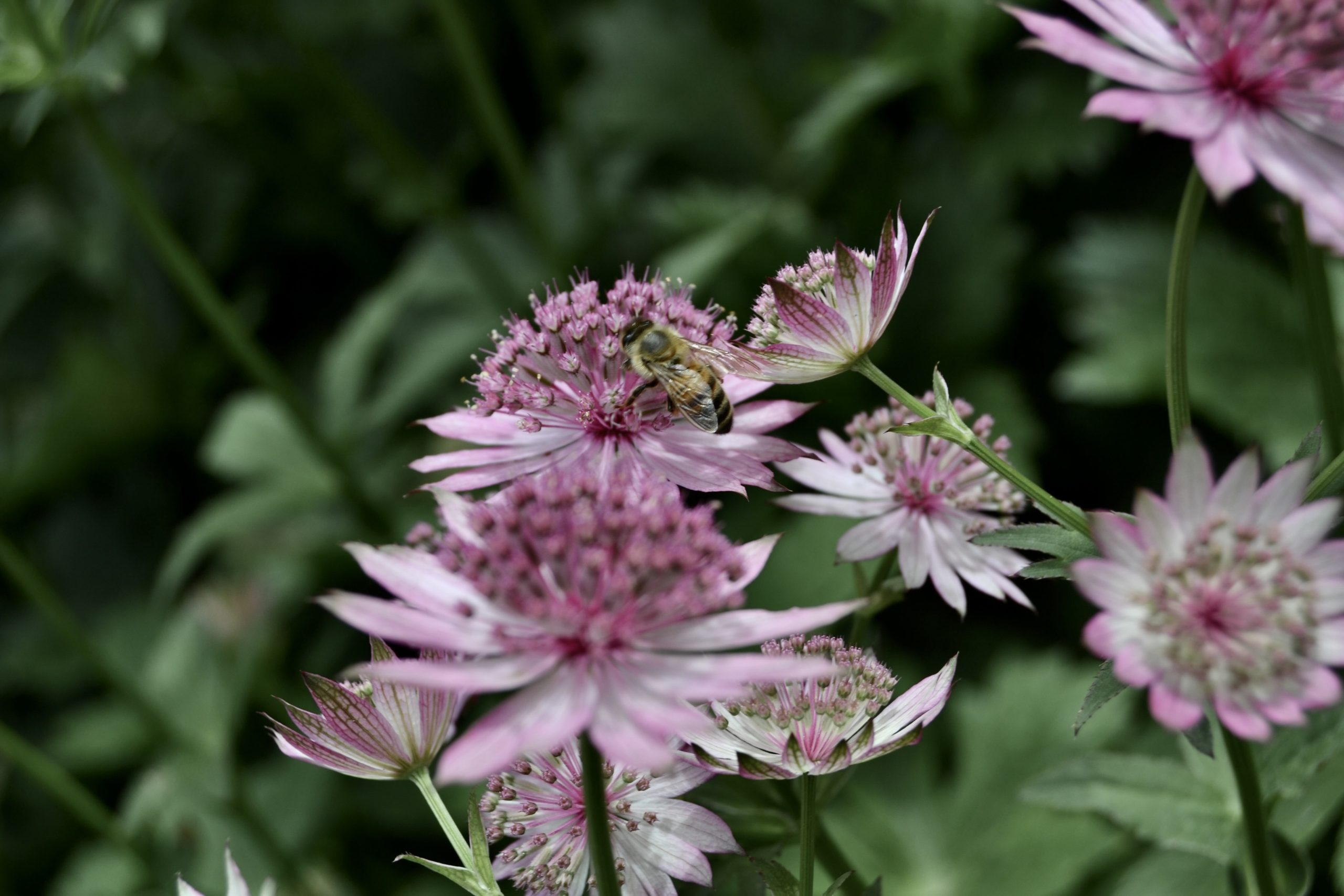
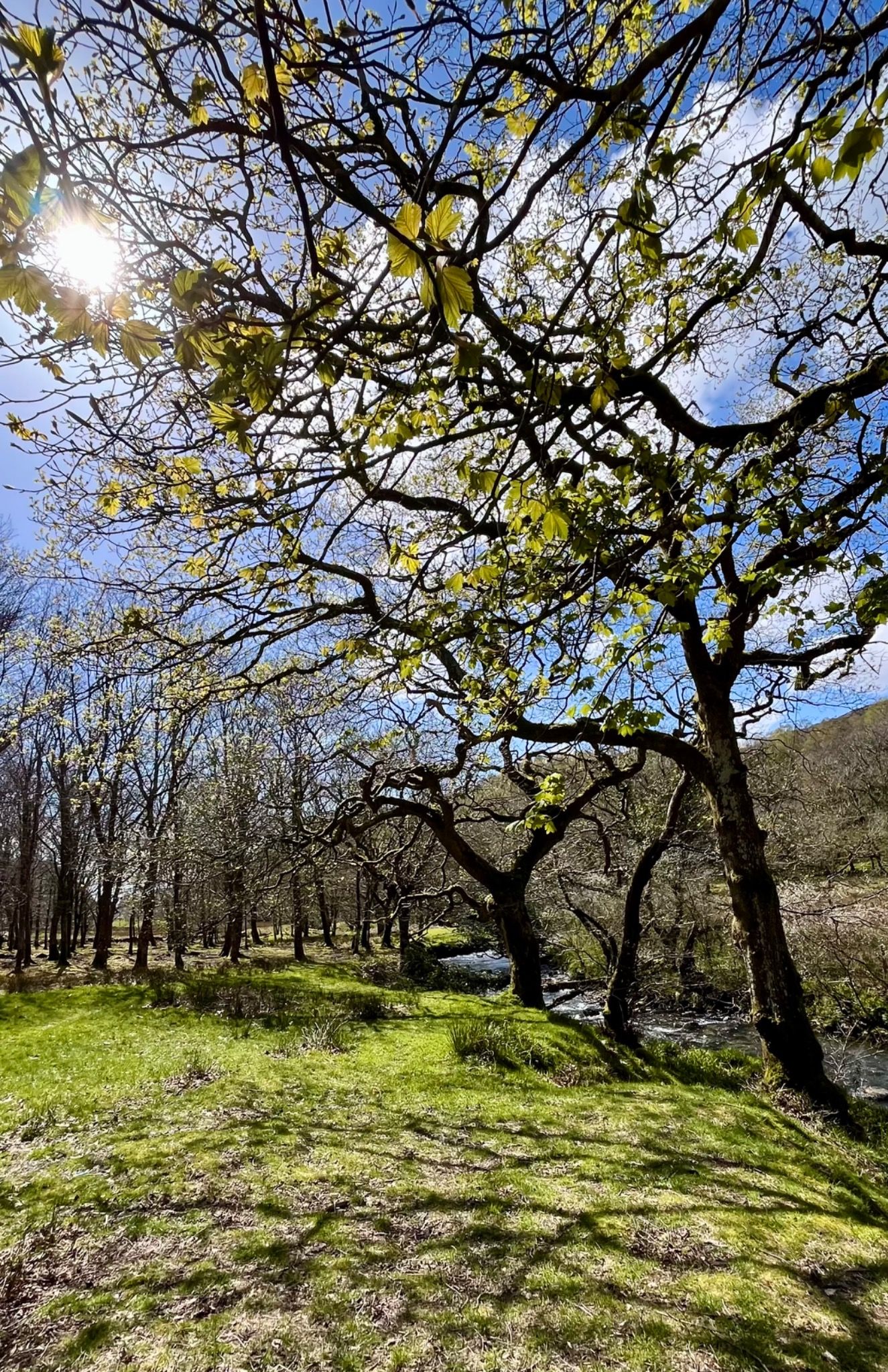
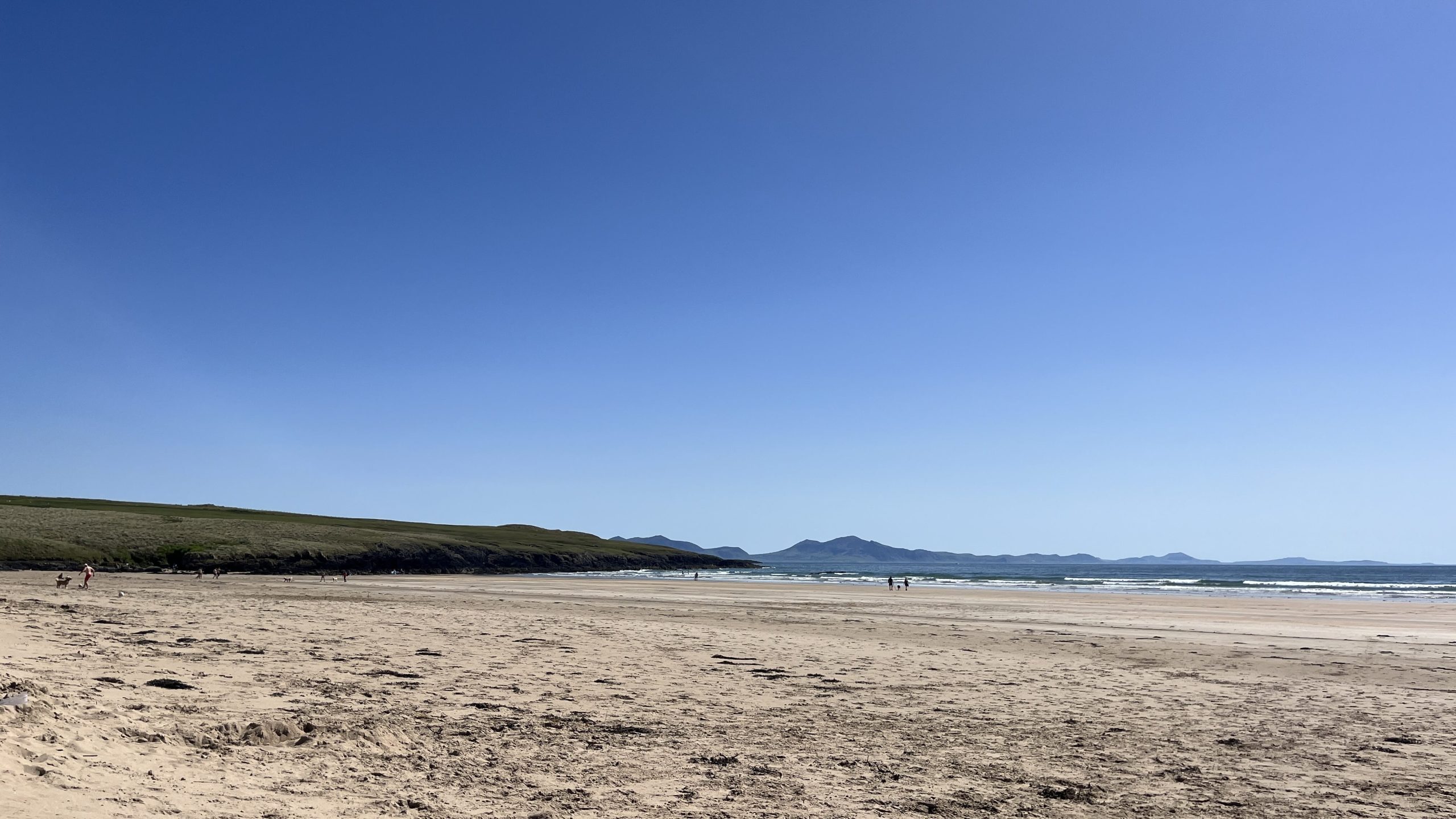
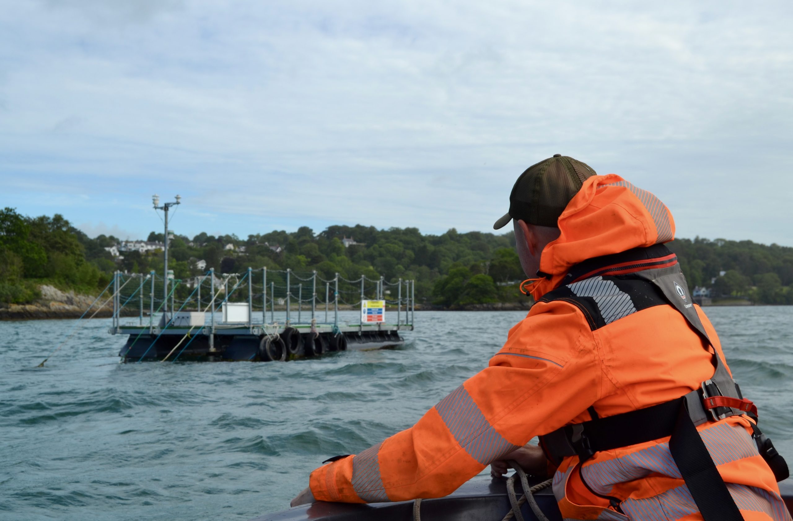
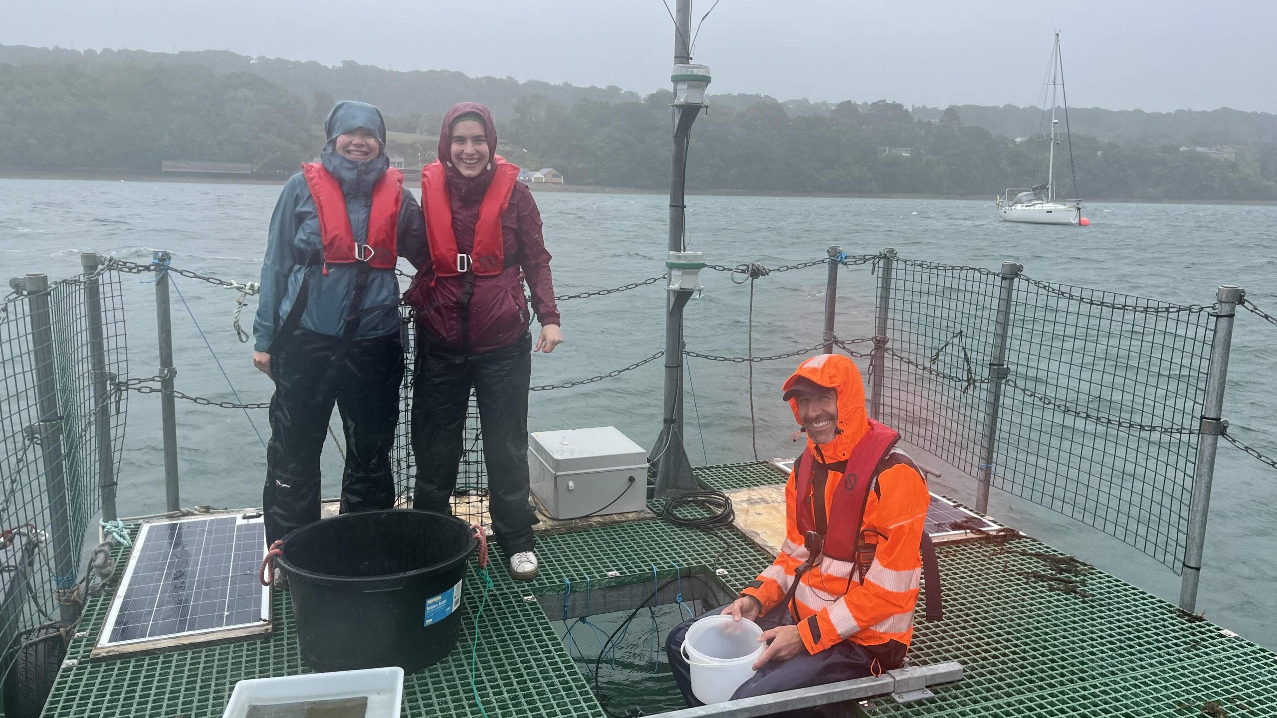
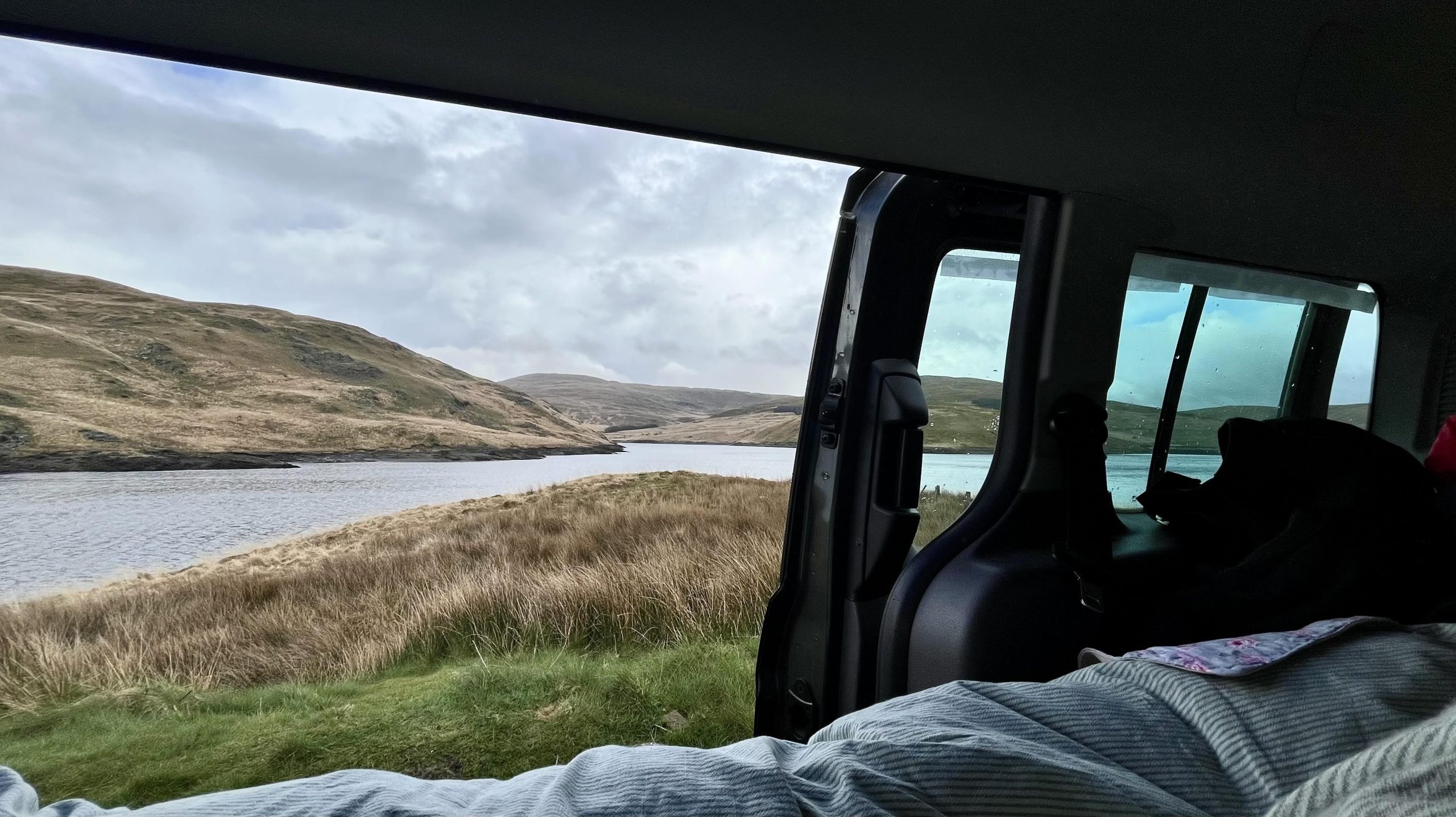
Hello from Wales, more precisely, from the Isle of Anglesey in the north of Wales. Here lies the School of Ocean Sciences (SOS) directly at the Menai Strait, where the ocean changes direction by 180 degrees four times a day. My name is Agnes, and I study Environmental Engineering in Munich and have decided to explore a new scientific topic with the GAME project. For someone like me, who is strongly interested in marine biology, it was quite a piece of luck to end up in a place with this high marine biodiversity. Every day, it seems like the sea breathes in and out – but mostly out as it is quite windy here, like a fresh salty breeze going through your hair.
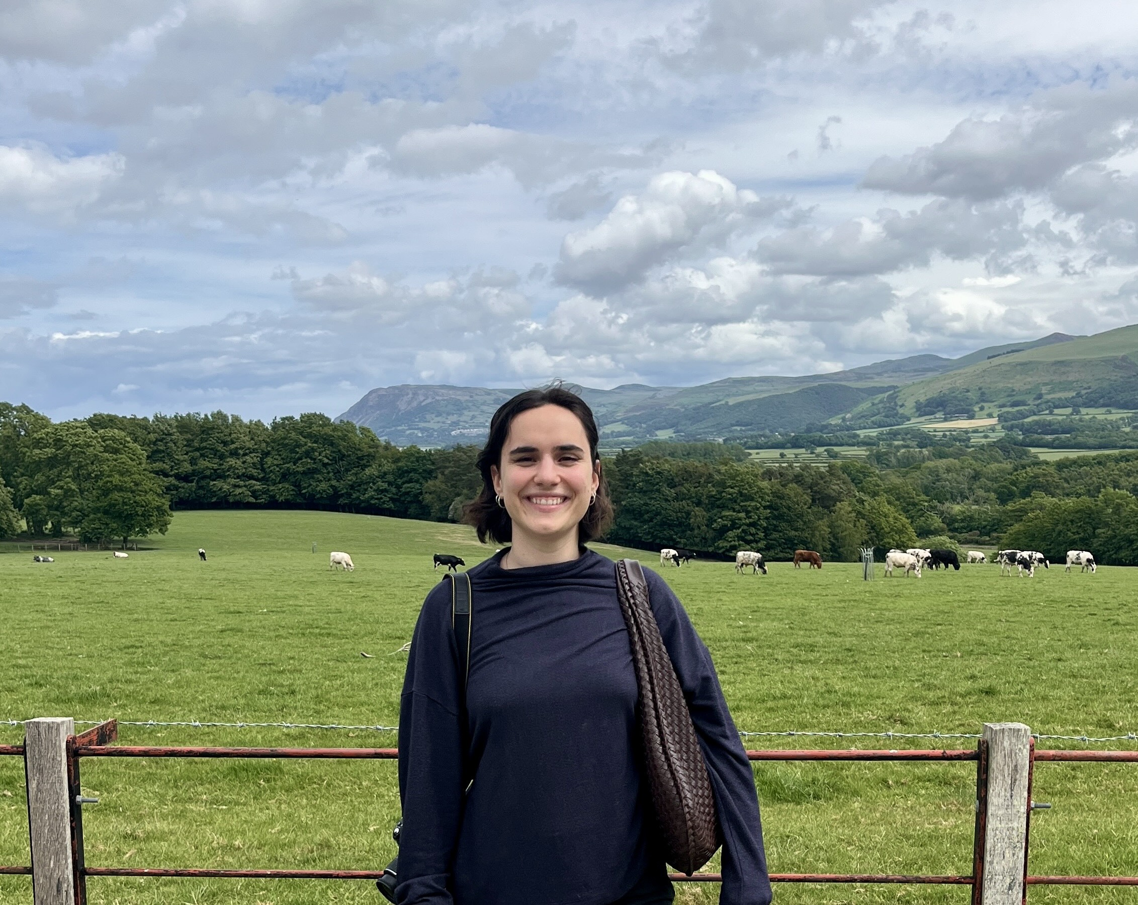
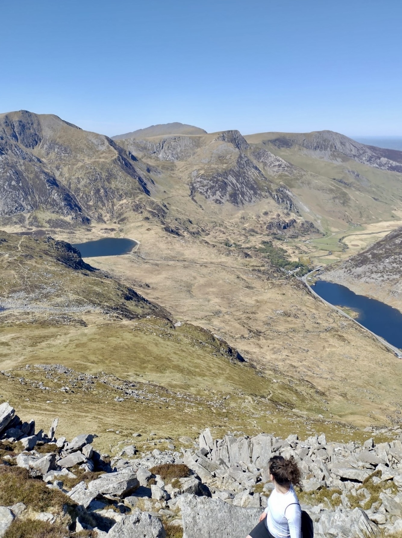
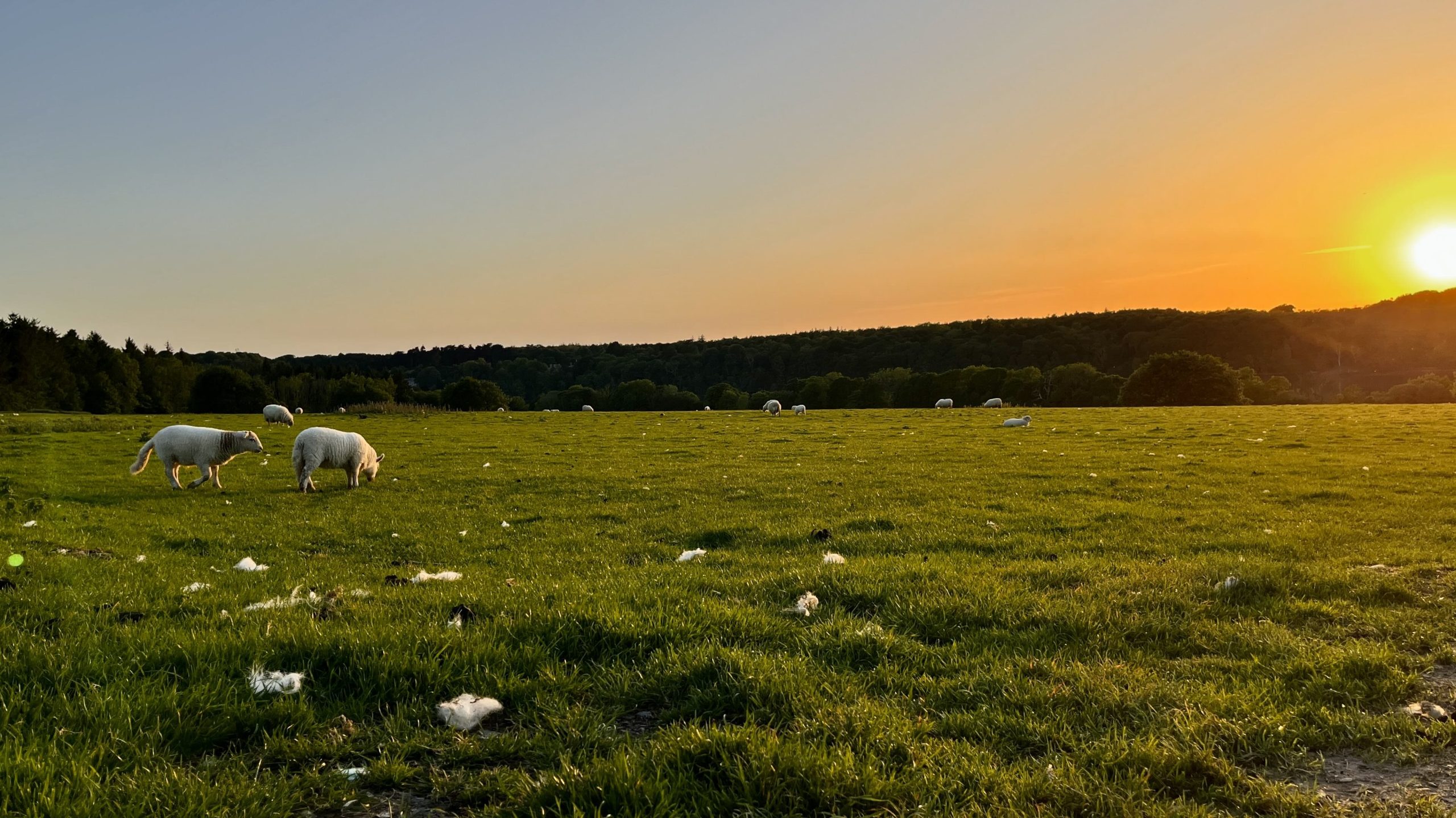
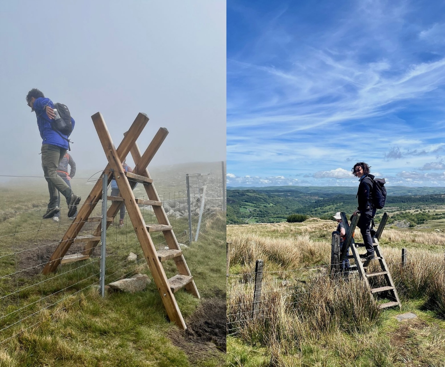
Before arriving here, I never imagined that the nature in North Wales is such a mysterious beauty. It does welcome you to sit in the forests and watch the wind weave its way through the trees, rustling the leaves and casting shifting patches of sunlight across the moss and undergrowth. Sometimes you can hear the calls of birds echoing above, and the scent of damp earth and pine is carried through the air. Or you might walk across rolling green fields speckled with grazing sheep and wildflowers, then reach the rocky coastline where the sound of waves crashing against cliffs rises to meet you. Within minutes, you can watch the deep blue sea stretching below or observe the silver shimmer of sunlight on the water. If you want to experience some lonely time in nature, that’s your place to be. When the deep-hanging clouds allow it, you can even see the mountains with their peaks often veiled in mist, waiting for your visit. There is a certain calmness to the landscape that envelops you, encourages you to be mindful. But let’s take a break from my romantic view of non-cultured nature and give you some information about the life and work here.
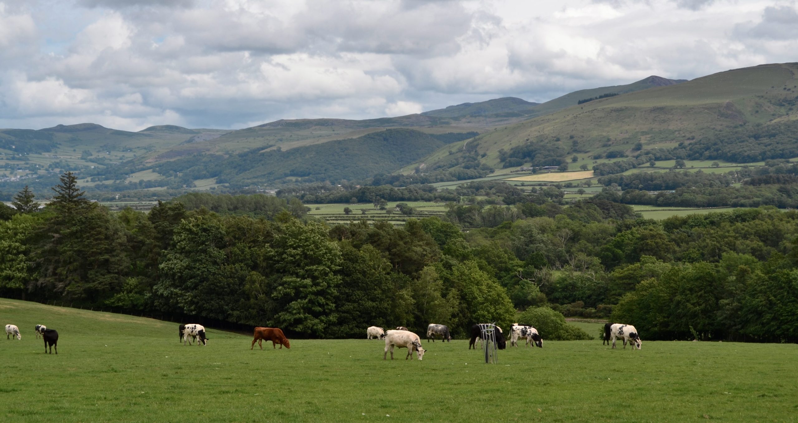

Now, I live in Bangor, right next to a natural reservoir, perfect for running or just a slow walk to say goodnight to the sun and the cows who live there. But be careful, it is hilly in Bangor, even though I love to have a walk, the walk up the hill from the city back home takes a while. With the wind and respect to the hilly topography, I sometimes think about what it would be like to be a bird. It seems a perfect place for it.

Many people asked me about the weather before I came here. Wales has a reputation for rain, wind and clouds, but so far, the reality I experienced has been quite different. April and May had been surprisingly sunny and somehow dry. However, locals keep reminding me that summer is still coming. During a hike, one colleague quoted her mother saying, “There is no bad weather, rain just makes the hike more atmospheric.” As a German, I can only agree to this philosophy.
The people at the School of Ocean Sciences are just as welcoming as you can expect from the British. Everyone is willing to help, answer questions, and share ideas. The technical staff, Pete, Aled, and Steve, already provided invaluable support to me while I was planning and building the experimental mesh cylinder. Alice, a marine biologist who volunteers on the project, has also become a great help. Her expertise in identifying marine organisms perfectly complements my background in environmental engineering. My main supervisor, Svenja, and I meet regularly to discuss the progress of my work and solve the inevitable challenges that arise during a field experiment.

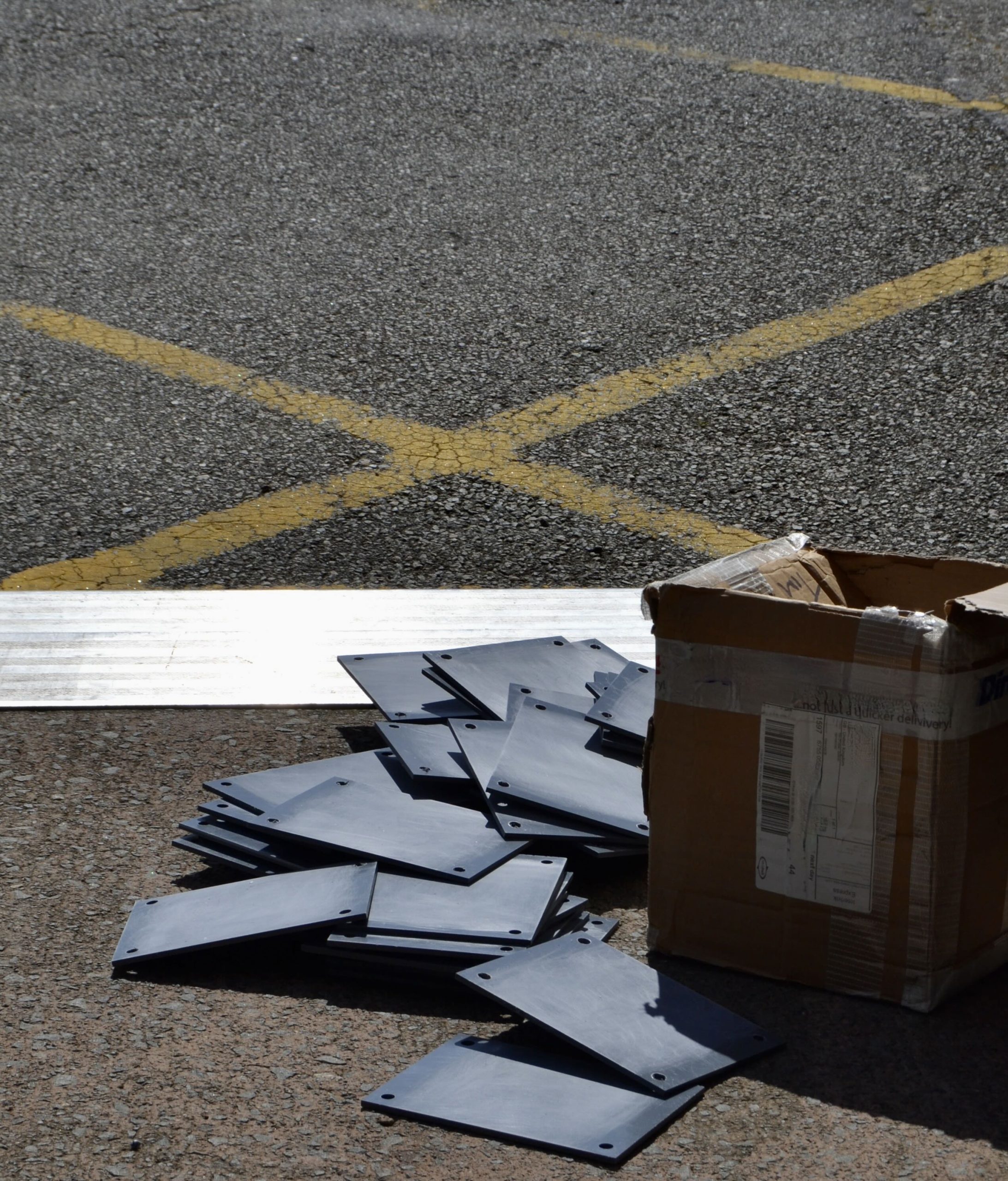
Speaking of challenges, I need to mention that, for me, this year’s GAME project is slightly different from the other participants’, as I do not have a team partner. This year’s project examines how underwater soundscapes, such as boat noise, or natural habitat sounds influence the species composition and abundance of sessile marine invertebrates. Each of the two active sound treatment levels plays at a specific temporal rhythm for 2 or 3 months, depending on site-specific restrictions. If there are two team members, then each chooses one of those treatment levels for their experiment. For comparison, there is always an additional treatment level, the ambient control. To ensure the project is feasible while maintaining research quality, I chose to focus on only two sound treatment levels: anthropogenic noise and the ambient background soundscape as the control. Hence, over the next three months, I will use underwater speakers to play back boat noise to simulate exposure to an anthropogenic soundscape at one of my two study sites. At the other site, no additional sound will be added to the existing ambient soundscape.
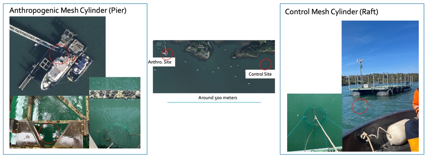
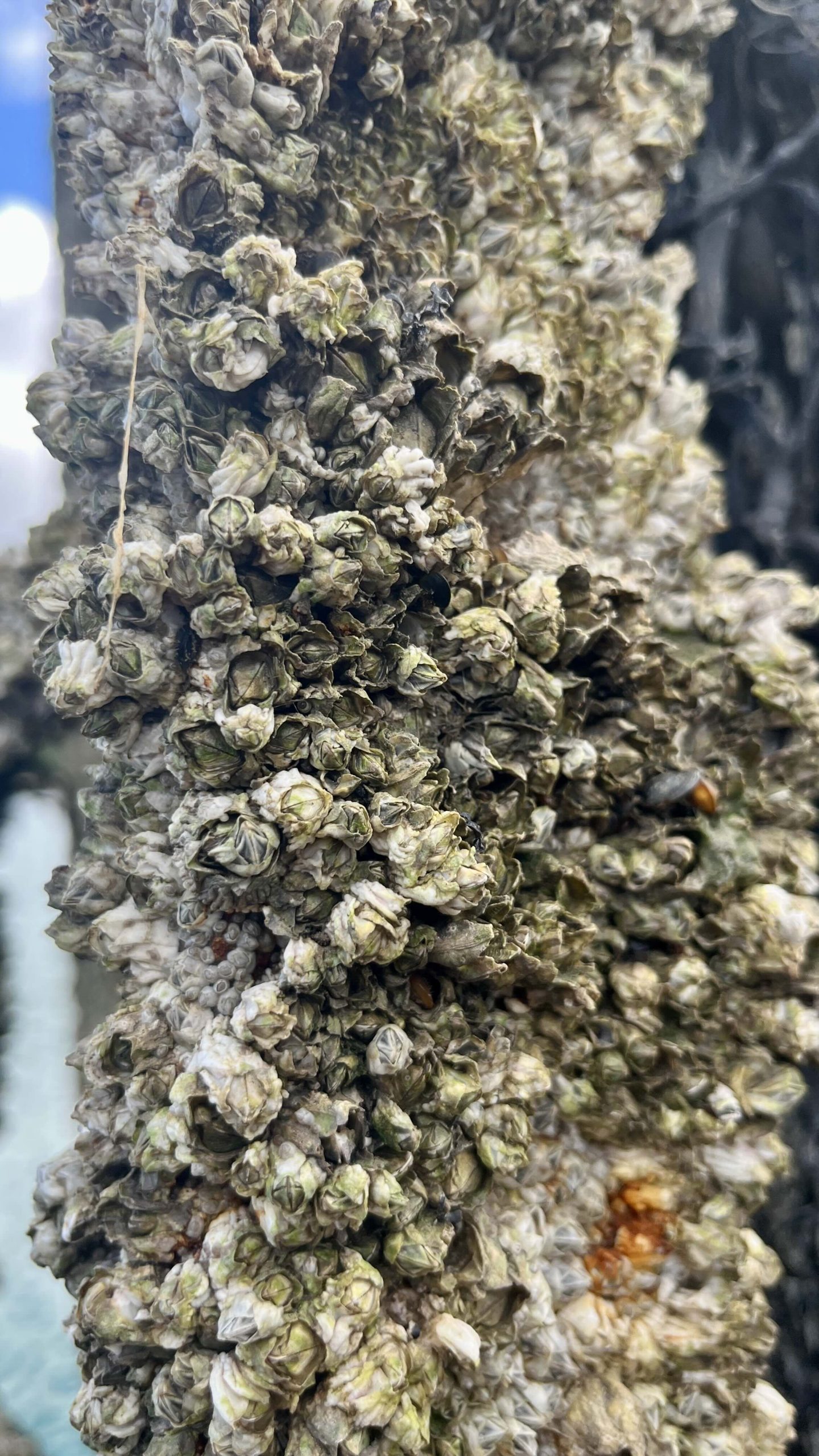
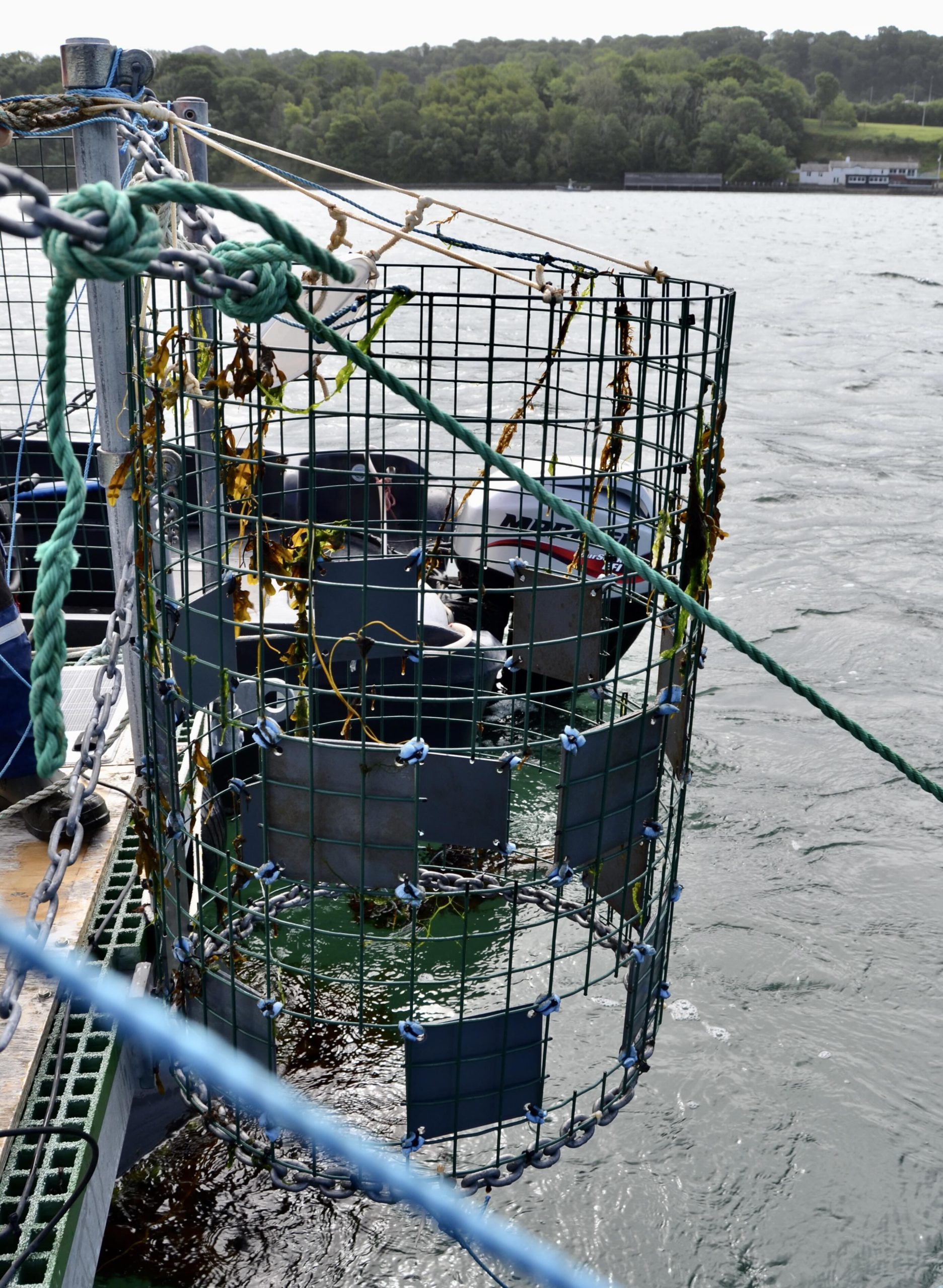
This experimental design allows me to examine whether differences in underwater sound conditions influence the settlement and growth of marine sessile organisms that attach to hard surfaces such as rocks or, as a substitute, settlement panels. My two experimental sites are located 500 meters apart to ensure acoustic isolation, meaning that the boat-noise playback will not influence colonisation at the Site of the Control Frame (Raft). However, as I am investigating whether boat noise influences community composition, it is essential to ensure that the two experimental sites do not differ substantially in their initial species pool. To assess this, I deployed larval-pool test panels for two weeks before the start of the experiment and identified the species that colonised them. Statistical analyses of these communities, together with information from previous studies conducted at the same locations and accounting for the unique tidal dynamics of the Menai Strait, enabled me to evaluate whether both sites experience comparable environmental conditions and larval supply.
The Menai Strait itself is shaping the local environment and is influencing the practical aspects of my research. Functioning as a channel that separates Anglesey from mainland Wales, it features tidal reversal. During these tidal shifts, water flows in opposing directions at different times, so that as the tide comes in, some water moves toward the strait’s central point. In contrast, simultaneously, other water recedes in the opposite direction as the tide goes out. This situation is comparable to a river that changes direction several times per day in response to the tides. But instead of being one river, the Menai Strait is more like two rivers that meet in the middle of the strait. Furthermore, the Menai Strait experiences some of the largest tidal ranges in the world, with a difference of up to 8 meters between low and high tide. On a personal level, I learned that misjudging the tidal schedule can make it difficult, or even impossible, to retrieve equipment, underscoring how closely the natural dynamics of the Menai Strait are intertwined with the day-to-day realities of conducting fieldwork here.
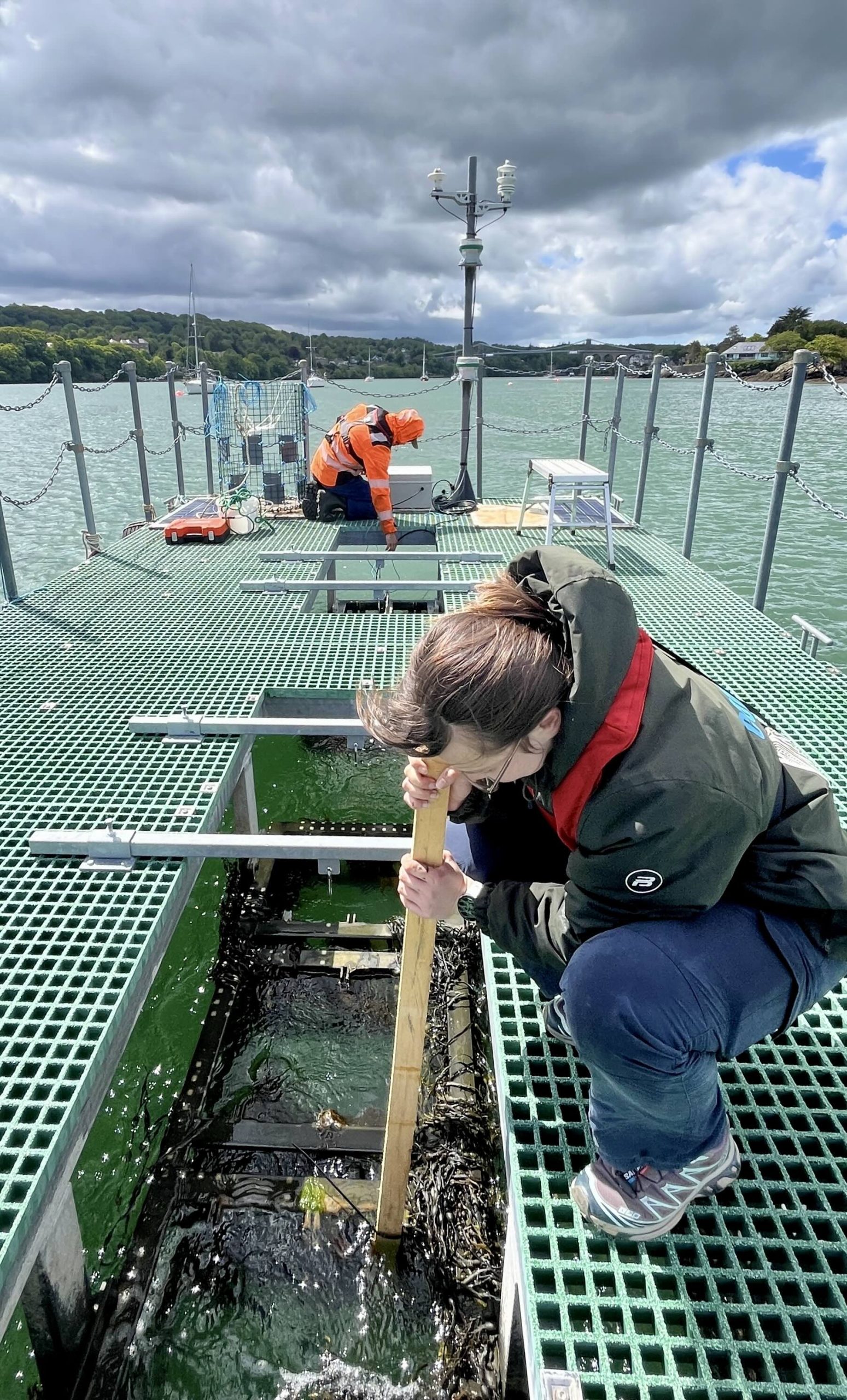
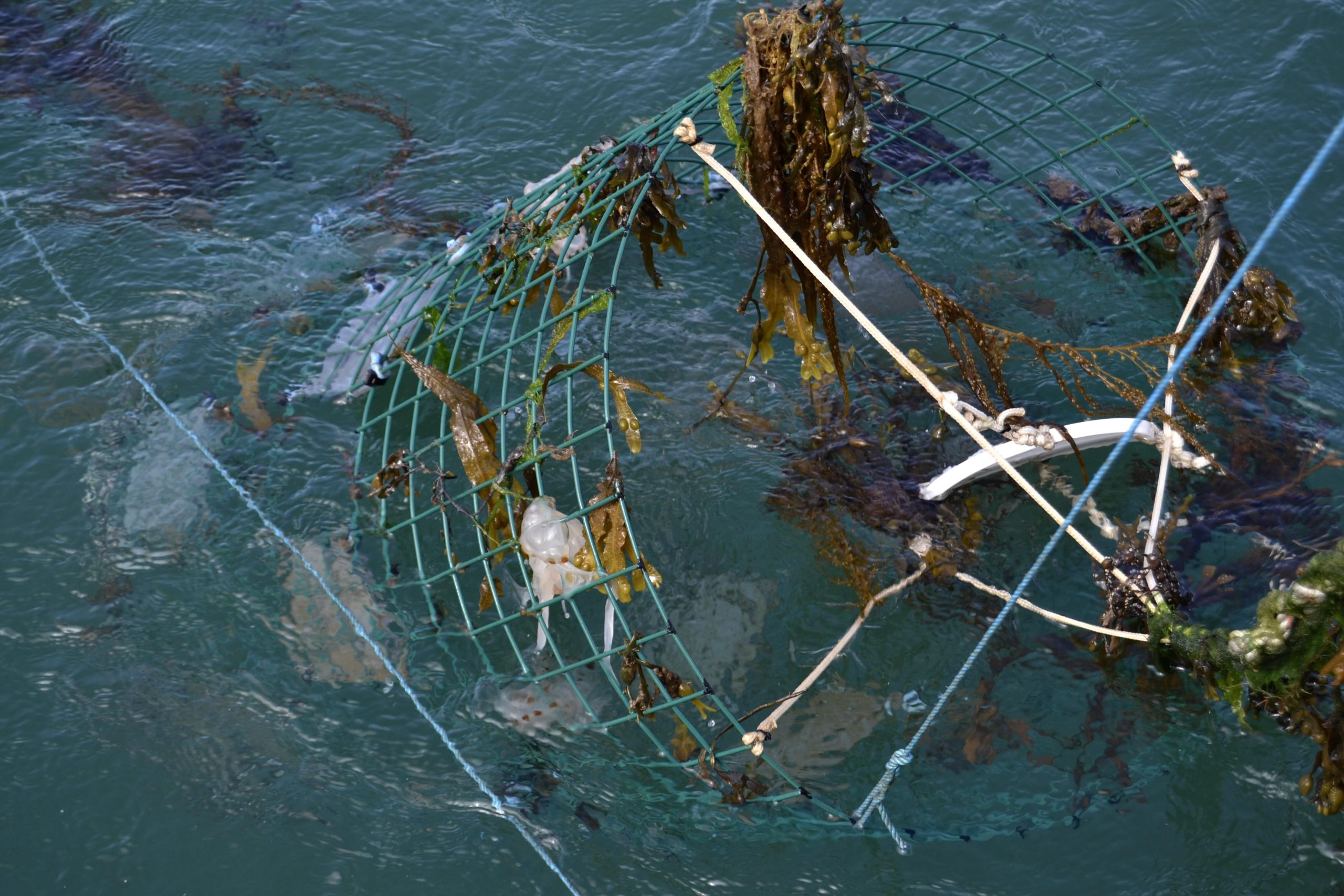
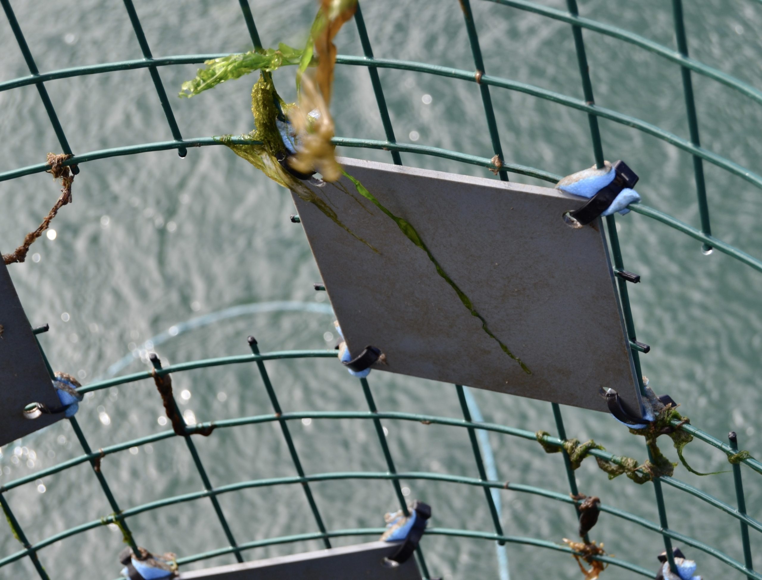
Alongside the sound experiment, I am deploying additional recruitment panels, which are replaced with empty panels every two weeks. The retrieved panels are transported to the laboratory, where Alice and I identify the newly arrived species. This tracks which colonisers are present in the water column at different times during the experiment, and it is always a surprise which new species are on the panels. One of the most rewarding aspects of the project is the opportunity to see ecological processes unfold over time. Looking at the small, settled organisms through the microscope is like peeking into another world. So far, the panels are full of tiny hydrozoans, barnacles, bryozoans and tunicates.
Being responsible for the experiment in Wales on my own gives me many opportunities to learn and grow as a scientist. I have gained experience in logistics planning, organising fieldwork around tidal cycles, constructing equipment, processing samples, and managing acoustic and biological datasets. I never thought there would be so much planning required for a single site-specific experiment, especially since the theoretical preparation had already been completed during the course in Kiel. Nevertheless, this experience has left me with a long to-do list and many opportunities for further learning. One advantage is the opportunity to work closely with other team members on the GAME project and engage in meaningful exchanges. Whether discussing similar or contrasting challenges, finding solutions, or sharing personal experiences, it is important to both offer advice and share your experience working on an international project, just as much as you receive guidance from others.
At the moment, the experiment is fully underway. The mesh cylinders are in the water, the sound playback is running, and the first settlement panels have been analysed. Over the next few months, I will analyse species, check the sound system, and try to start writing my master’s thesis. Wish me and my little invertebrate’s luck!
I am enjoying life in Wales, learning some new things every day, about British history and environment, and trying to make it up Bangor’s hill. Between the strong tides, the endless shades of green and the ever-changing skies, it is hard not to enjoy the nature of the north of Wales.
From Desert to Seafloor

Fig. 1) team Strata That Matta: Victoria C., Maeghan D., Maddie B., Vale B. (from left to right)
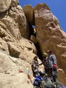
The months leading up to OCEAN CORE Academy were filled with another type of adventure for me, surveying the badlands of New Mexico in search of dinosaur bones. Yet, my work in the Gulf Coast Repository consisted of examining ocean cores using a microscope. Although these experiences couldn’t be any more different, the two were similar in that each attempted to answer the same question: what did Earth look like in the past?
I focus much of my research on vertebrate paleontological and geological fieldwork, such as prospecting for fossils, measuring strata, or describing ancient paleoenvironments and faunal assemblages. While I knew about microfossils, I had not fully grasped how much geological history is present in them.
Fig. 2) fieldwork, NM (May 2026)
History Through a Microscope
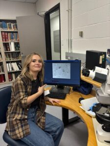
This leads me to one of the most memorable parts of OCEAN CORE Academy, learning to prepare smear slides and identify what existed within the ocean cores. Ocean sediments are fairly recent in that they have not yet been lithified, each layer represents tens to hundreds of years of depositions onto the seafloor. What I looked at was much deeper!
It was a momentous occasion when I first saw a radiolarian beneath the microscope! These tiny fossilized organisms provide surprisingly detailed insights into ancient environments. The conditions in which different groups of microfossils thrive vary, but by tracking how they fluctuate between layers, we can reconstruct climatic shifts over geologic time.
Team Strata That Matta correlated a transition from calcareous to siliceous ooze layers with a cooling climate!
Fig. 3) my first time seeing microfossils
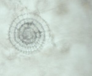

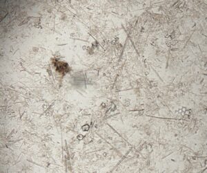
Fig. 4) radiolarian Fig. 5) coccolithophores Fig. 6) sponge spiccules
Bringing OCA Back to AZ
Upon my return to Arizona, I will carry this new perspective with me. As I move forward with future projects and field seasons in New Mexico, volunteer at the Arizona Museum of Natural History, and pursue my degree, the skills I developed here will prove to be invaluable for strengthening my own research.
Prior to attending OCEAN CORE Academy I viewed microfossils as existing, yet somewhat separate from my projects. This place has challenged that perspective. I came to understand that many of the most detailed records of Earth’s past are the microfossils hidden within a single grain of sediment!
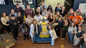
Fig. 7) class of OCA 2026
Written by OCA 2026 student, Maddie Baare


-
Climate Change11 months ago
Guest post: Why China is still building new coal – and when it might stop
-
Greenhouse Gases11 months ago
Guest post: Why China is still building new coal – and when it might stop
-

 Greenhouse Gases2 years ago
嘉宾来稿:满足中国增长的用电需求 光伏加储能“比新建煤电更实惠”
-

 Climate Change2 years ago
嘉宾来稿:满足中国增长的用电需求 光伏加储能“比新建煤电更实惠”
-
Climate Change2 years ago
Bill Discounting Climate Change in Florida’s Energy Policy Awaits DeSantis’ Approval
-

 Renewable Energy9 months ago
Sending Progressive Philanthropist George Soros to Prison?
-

 Carbon Footprint2 years ago
US SEC’s Climate Disclosure Rules Spur Renewed Interest in Carbon Credits
-
Greenhouse Gases12 months ago
嘉宾来稿:探究火山喷发如何影响气候预测