
This blog was written by Kassidy Troxell, Ph.D., a Research Assistant Professor at Florida international University’s Institute of Environment, and collaborator with Ocean Conservancy on our work to promote healthy Florida aquatic ecosystems. Dr. Troxell is a lead scientist executing the nitrogen fingerprinting discussed in this blog.
November was Manatee Awareness Month, a month dedicated to highlighting the popular aquatic mammal and the broader importance of clean, healthy waterways in Florida. One of the greatest challenges to water quality in areas like Tampa Bay is nutrient pollution. Excess nutrients in coastal waters fuel harmful algae which “bloom” into patches, one example is the well-known Karenia brevis referred to as red tide, causing fish kills and human respiratory problems while also reducing the sunlight needed by underwater seagrasses to flourish. These blooms diminish essential seagrass habitats, impacting marine species like manatees, harming local ecosystems and affecting human health. Identifying the primary sources of nutrient pollution is crucial for developing targeted strategies to control nutrient levels and maintain the health of delicate ecosystems.
Love ocean content?
Enter your email and never miss an update
In Tampa Bay, my lab at Florida International University has partnered with Ocean Conservancy to do just that: understand and address nitrogen pollution, the nutrient that contributes to water quality impairment, in the Hillsborough Bay and the larger Tampa Bay ecosystem. By using manmade or commonly used chemicals, we can pinpoint the sources of nitrogen—whether from untreated stormwater street runoff, treated home, business or industrial wastewater, or agriculture—allowing for more targeted management efforts. Just as each of us humans have our own unique fingerprints made of various patterns and distinctions, contamination sources have a unique makeup of compounds that allows us to fingerprint and track their movements throughout a watershed.

Key findings from recent study in Tampa Bay
The Hillsborough River, which flows into Hillsborough Bay and is vital to the health of Tampa Bay’s ecosystem, serves as the geographic focus of our study. Our preliminary results reveal that nitrogen levels in these waters rise significantly during the wet season when runoff is at its peak. Chemical tracers, which act like “markers” for pollution sources, suggest that reused non-drinkable treated water (reclaimed water), stormwater and agriculture are contributing sources of nitrogen into the waterway. Within the Hillsborough River watershed, nitrogen levels show distinct patterns (i.e., “fingerprints”) linked to various sources: reclaimed water and agricultural activities are prominent in the upper watershed, while urban stormwater runoff and wastewater inputs are notable near the river’s mouth. Potential contributions from other sources, such as septic systems, are still under investigation.

Now that we have identified the preliminary nitrogen sources and hotspots, the next phase of the project will focus on the sources that are contributing the largest nitrogen loads, the geographic origins of those sources and the amounts of the nitrogen going into the waterways. Future sampling will expand sampling sites in the tributaries that feed into the preliminary hotspot locations along the mainstem (the primary downstream river segment in contrast to its tributaries). This information will help tailor interventions to reduce nitrogen loads at the source and guide management efforts to improve water quality and ecosystem recovery in Tampa Bay.
The future of Florida’s water quality
Our research underscores the need to better manage nutrient levels to protect Florida’s coastal waters. The data generated from our study will give policymakers a more precise geographical understanding of nitrogen hotspots for prioritizing actions to curb nutrient pollution. Indeed, Ben Albritton, the incoming Majority Leader of the Florida state senate, recently said as much when he pointed to the importance of fresh, accurate data needed to drive solutions, whether these are new policies, investments or on-the-ground management practices.

Our activities on land—whether through treated wastewater, stormwater runoff or agricultural practices—have direct impacts on coastal ecosystems. While the Hillsborough River is the focus of this pilot study, we believe the nutrient fingerprinting techniques will be a valuable water quality management tool in other Florida estuaries and bays as well. By pinpointing and quantifying the largest nutrient sources, we can better protect the health of our marine environments and communities alike, which will benefit all Floridians.
Undoubtedly, Florida’s waterways are facing enormous challenges. Ocean Conservancy is dedicated to addressing nitrogen pollution, in part, for marine species like manatees that are so greatly impacted by threated water quality. Take action with Ocean Conservancy to demand greater protections for imperiled manatees and improvements in water quality in Florida and beyond.
The post Fingerprinting the Source of Nitrogen Pollution in Tampa Bay appeared first on Ocean Conservancy.
Fingerprinting the Source of Nitrogen Pollution in Tampa Bay
By Tina Hans (GEOMAR)
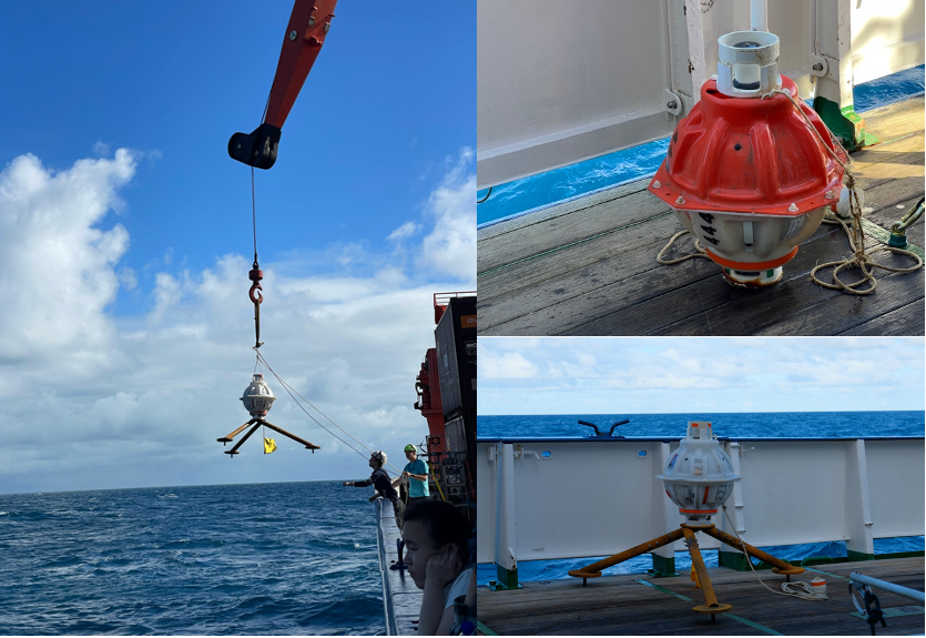
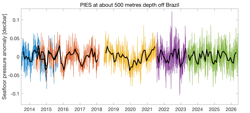
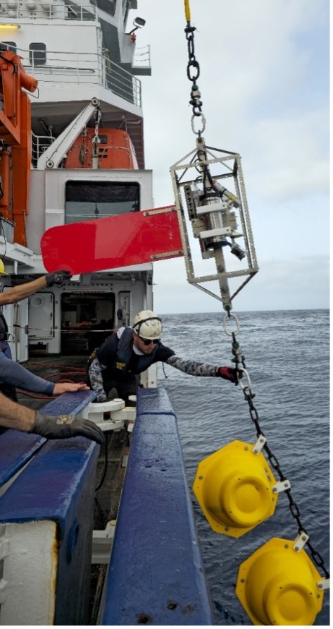
One main objective of the cruise is to investigate the large-scale ocean currents in the tropical Atlantic. For that purpose, we are maintaining several long-term observatories at the seafloor and in the water column. Additional to the moorings which have been described in the previous blog “Keeping the record alive”, we deployed and recovered close to the Brazilian coast so-called PIES. They have – as some might say unfortunately – nothing to do with pastries but are oceanographic instruments that measure the pressure at the seafloor as well as the time an acoustic signal takes to travel from the instrument to surface, where the signal is reflected, and back. We deployed six of those instruments across the continental shelf off Brazil at depth ranging from 150 metres to 3000 metres. These deployments are the result of a collaboration with the University of Bremen. We also successfully recovered one PIES that spent just over three years at the seafloor at a depth of 500 metres. With the data of the recovered PIES, we could extend our time series of seafloor pressure measurements at 500 metres depth. This time series, which goes back until 2013, spans now 13 years.
This still leaves the question of what the pressure at the seafloor can tell us about ocean currents. To answer this, one needs to know that the ocean dynamics are largely governed by a balance of two physical forces: the pressure gradient force and the Coriolis force. Essentially, when water ‘piles up’ somewhere, a current is created which attempts to even out the differences, and the direction of this current is deflected due to the Earth’s rotation. This force balance can also be used to directly relate the difference in pressure between two locations to the mean velocity in between these locations. We make use of this relation by measuring the seafloor pressure not just off Brazil but also off Angola at a similar latitude. With the combination of these measurements, we can calculate the mean north-/southward velocities across the Atlantic between Brazil and Angola. From this velocity we can then derive the strength of the Atlantic Meridional Overturning Circulation (AMOC).
However, there is one caveat: the pressure sensors are drifting over time. This makes it impossible to make statements about long-term trends, but we can still make statements about the seasonal to interannual variability of the AMOC. Therefore, the measurements of the PIES can be used to better understand the large-scale currents in the tropical Atlantic. In a next step, we are now using these measurements to better understand the linkage of the AMOC to climate variability in the tropics.
By Qi-Fan Wu (Niels Bohr Institutet, University of Copenhagen)
During our journey, we saw many beautiful cloud patterns while looking outside the METEOR! Even though people do not always pay attention to them, clouds are among the most visible elements of the sky and naturally form part of our everyday background. And when we sailed away from the coastal region of Recife to the open ocean, the sky seemed to open up, allowing clouds to reveal their full variety and structure.
In climate modelling, clouds are one of the biggest sources of uncertainty. There is a famous saying in mathematics: “Mathematics is the queen of the sciences, number theory is the crown of mathematics, and the Goldbach Conjecture is the pearl on the crown.” The same idea can be applied to the study of clouds in Earth science. There is still no general macroscopic theory of clouds. Cloud physics is an absolutely fascinating topic, as it combines turbulence, stochastic processes, chemicals in the air, multiscale interactions within the Earth–atmosphere system, and a close connection to our daily weather.
In this blog entry, we would like to share some lovely photos of cloud patterns that we took on METEOR. Instead of serious systematic investigations, we focus on the basic cloud physics behind some typical cloud phenomena shown in these photos. These examples might provide something interesting to think about during our leisure time, even after returning to land. If nature is an artist, clouds are among its finest masterpieces, shaped by physical laws and stochastic processes.
What are clouds, and what is inside them? Clouds are made of many liquid water droplets and ice crystals inside the boundaries of the cloud. They are mostly air, with the many particles dispersed widely and more or less randomly throughout the cloud interiors [a]. The individual particles that make up a cloud are very, very small and not generally visible to the human eye.
When we look up from our research vessel METEOR and observe clouds, we first see their macroscopic structure: their overall shape, height, thickness, and organization across the sky. Broad, layered clouds often form through slow, large-scale ascent, while towering clouds with visible turrets reflect rapid rising motion in smaller air parcels. These visible forms are continuously shaped by moisture supply, cooling, turbulence, mixing with drier air, and precipitation, linking the large-scale atmospheric flow to the clouds we observe [a,b].
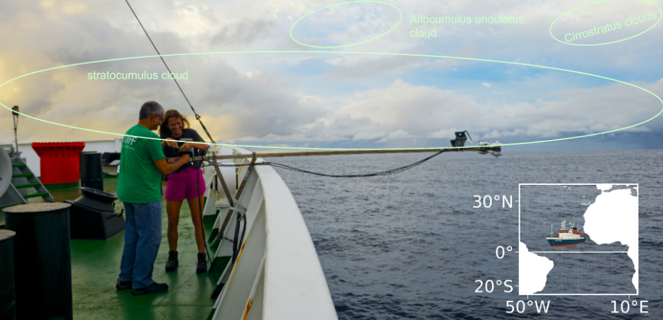
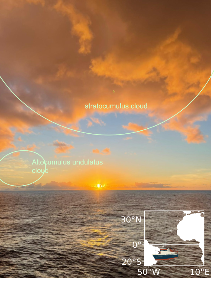
After leaving Recife, we entered a region typically influenced by the southeast trade winds of the tropical South Atlantic, where a vertically layered atmosphere, warm ocean conditions, and wind-driven mixing often promote a turbulent marine boundary layer. In Figure 1, the sky shows a layered cloudscape ranging from thin, high cirrostratus and altocumulus clouds to low cumulus and towering cumulonimbus clouds. These different forms reflect how the atmosphere organizes moisture, cooling, and vertical motion: broad layers are associated with gradual ascent, while the rising turrets of cumulus and cumulonimbus reveal stronger localized updrafts. Together, they illustrate the visible macroscopic structure of clouds, shaped by atmospheric motion and the microphysical processes occurring within them.
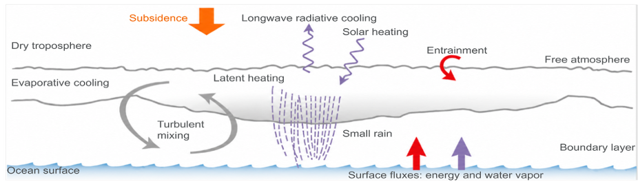
It should be noted that, in general, atmospheric temperature in the troposphere decreases with increasing altitude. Over the subtropical oceans, however, this is not the case. A relatively thin temperature-inversion layer lies above the subtropical marine boundary layer, within which temperature increases with height and the atmosphere is highly stable (Figure 2). Cloud occurrence above the marine boundary layer is relatively low in this region. The base of the trade-wind inversion is typically located at an altitude of approximately 1–2 km, separating the moist lower layer from the dry free troposphere [c].
This large-scale thermodynamic structure provides the environmental conditions under which clouds form and evolve. At the microscopic scale, however, clouds consist of particles: liquid water droplets, ice crystals, or a mixture of both. Clouds composed entirely of liquid droplets are commonly referred to as “warm clouds”, whereas clouds containing ice particles are classified as “cold clouds”. When liquid droplets and ice crystals coexist, the cloud is described as a mixed-phase cloud. However, the distinction between “warm” and “cold” clouds hinge on the phase of the particles, not on the temperature. The warm/cold distinction depends on the microphysical phase of the particles inside the cloud, which a normal naked eye observation cannot resolve.
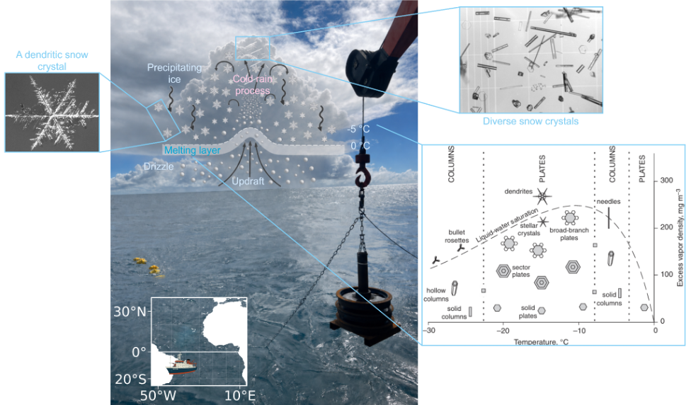
Warm clouds consist of liquid water droplets spanning a range of sizes, from small haze droplets and cloud condensation nuclei to cloud droplets, drizzle drops, and raindrops (Figure 3). Cloud droplets typically form when water vapour condenses onto cloud condensation nuclei. Rainfall develops when some droplets grow much larger: larger droplets fall faster, collide with smaller droplets, and collect them. As a result, many small cloud droplets can combine to form fewer, larger drizzle drops and eventually raindrops [a]. This process approximately conserves the total liquid-water mass within the cloud, while transferring water from numerous small droplets to a much smaller number of large drops that are heavy enough to fall as rain.
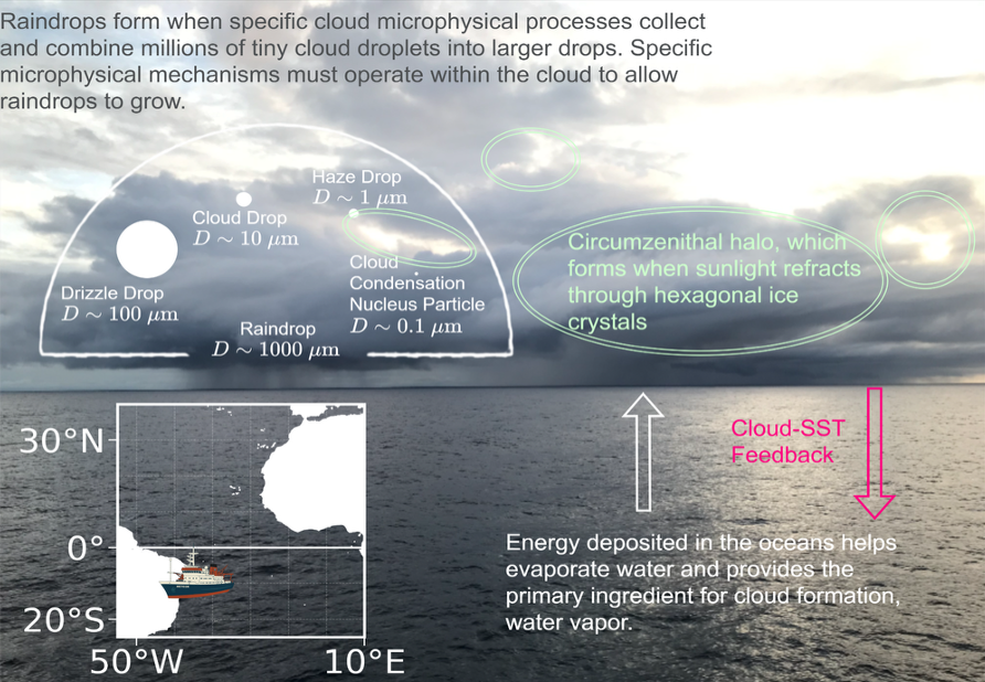
Cold clouds contain ice particles, either alone or together with supercooled liquid water droplets [a]. Unlike liquid droplets, which are nearly spherical because of surface tension, ice particles can develop a wide range of crystalline shapes, including plates, columns, needles, dendrites, and aggregates (Figure 4). Their shape depends mainly on temperature and ice supersaturation during growth by water-vapour deposition. As ice crystals become large enough to fall, they may collide and stick together to form snow aggregates, or collect supercooled droplets that freeze on contact, a process known as riming. The regular hexagonal structure of ice crystals can also produce optical phenomena such as halos, which form when sunlight is refracted or reflected by suitably oriented ice crystals in high-level clouds as shown in Figure 3. In mixed-phase clouds, uplift supports the growth of ice crystals at the expense of supercooled droplets. Once sufficiently large, the ice precipitates and may melt into rain or drizzle while falling through the melting layer (Figure 3).
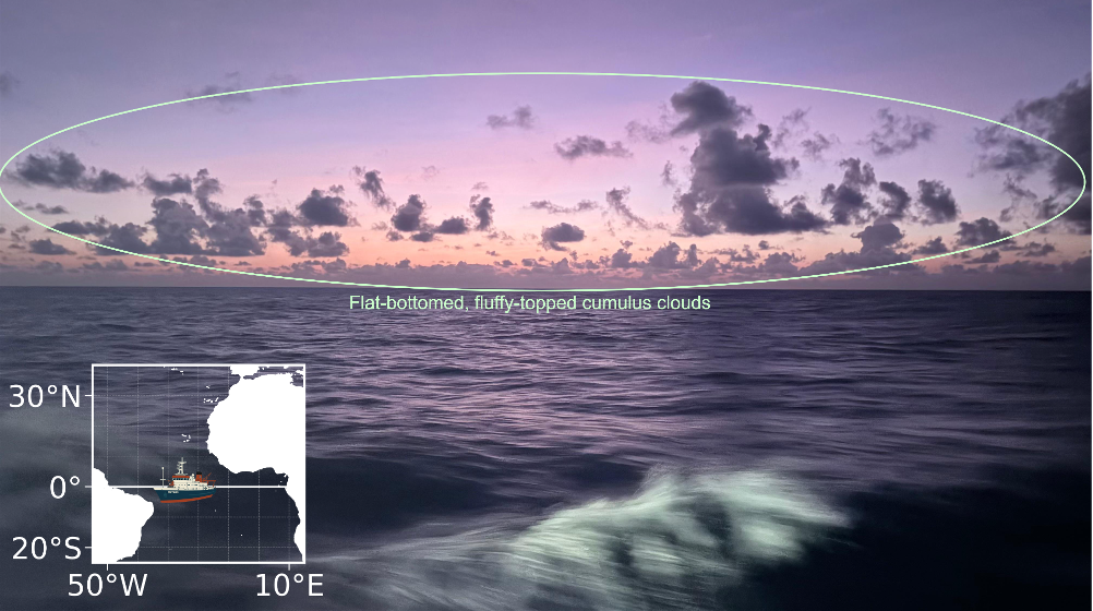
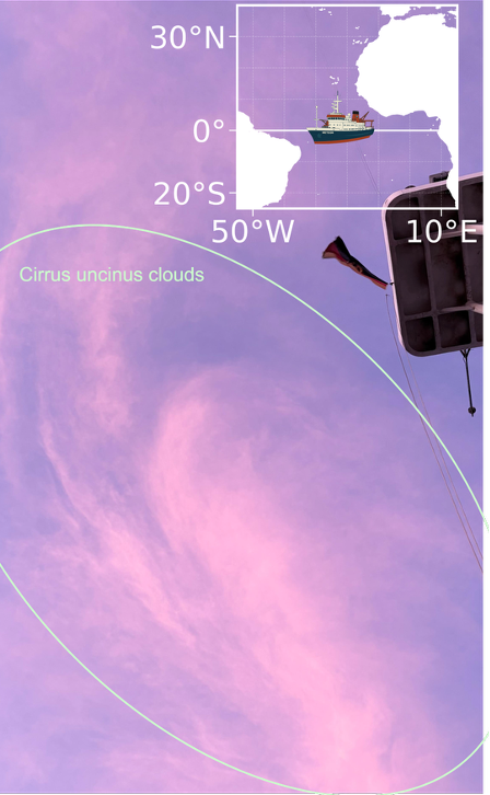
When we approached the equator, we saw many cumulus clouds with remarkably flat bases, marking the lifting condensation level where warm, moist air rising from the ocean cooled to its dew point and condensed into droplets. Similar temperature/humidity across an area leads to clouds sharing flat bases. Their uneven, towering tops reflected continued turbulence and convection above this level, revealing the active vertical mixing of the tropical atmosphere (Figure 5). As moist tropical air rises toward the cold-point tropopause, it encounters extremely low temperatures. When an air mass reaches a local temperature minimum, water vapour can freeze into very thin cirrus clouds (Figure 6).
After crossing the equator, we entered the Intertropical Convergence Zone (ITCZ), a band of heavy rainfall extending across the tropical Atlantic. Cloud organization within and around the ITCZ varies markedly from day to day. Extensive low-level stratocumulus clouds can also occur in the surrounding region, acting like a blanket that reduces the amount of incoming solar radiation reaching the ocean surface (Figure 7).
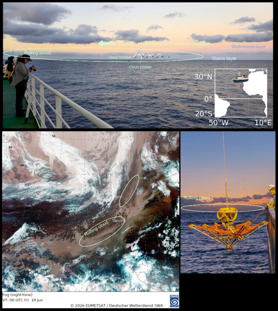
As we continued northward on our way home, we moved closer to the continent and witnessed some spectacular roll clouds, a very rare meteorological phenomenon. This type of cloud is known as “Morning Glory,” although evening land breezes can also produce roll clouds. The roll cloud is not attached to other clouds. associated with a solitary wave, a wave that has a single crest and moves without changing speed or shape.
As we were relatively close to the shoreline of West Africa, these roll clouds may have been produced by internal gravity waves propagating along a stable marine boundary layer [d]. The collision or sudden advance of a sea breeze or cold front can disturb the stable air layer near the surface, generating an atmospheric bore (a train of internal gravity waves). Such waves consist of alternating regions of upward and downward motion. Along the crest of the wave, moist air is lifted and cools to saturation, forming clouds, while behind the crest the air descends and warms, causing the cloud to evaporate. Because this cycle of ascent and descent extends along a long line of low-level convergence, cloud is continuously generated at the leading edge and dissipated at the trailing edge, maintaining a long, coherent band (Figure 8).
I think observing and thinking about clouds can be a nice hobby for enjoying the beauty of nature. Cloud processes are stochastic because nucleation and droplet collection do not occur at exactly the same time for every particle, even under the same environmental conditions [a]. Instead, freezing, condensation, and coalescence depend on chance microscopic events, so only some droplets become “lucky” and grow or freeze earlier than others. Perhaps cloud viewing could also give us good food for thought. After all, many cloud-related problems in climate modeling remain among the most beautiful mysteries in climate science.
Enjoy ~
References:
[a] Lamb D, Verlinde J. Physics and Chemistry of Clouds. Cambridge University Press; 2011.
[b] Levizzani, V., Kidd, C. (2025). Cloud Physics. In: Precipitation. Geophysics and Environmental Physics. Springer, Cham. https://doi.org/10.1007/978-3-031-97096-2_3
[c] Shang-Ping Xie. Subtropical climate: Trade winds and low clouds. In: Coupled Atmosphere-Ocean Dynamics. Elsevier; 2024. p. 139–163. doi:10.1016/B978-0-323-95490-7.00006-0.
[d] The Morning Glory and related phenomena. https://www.meteo.physik.uni-muenchen.de/~roger/AustralianProjects/TheMorningGlory/TheMorningGlory.html
By Naomi Krauzig (GEOMAR)
One of the most rewarding aspects of M219 has been contributing to the maintenance of the long-term GEOMAR mooring arrays that quietly monitor the tropical Atlantic year after year.
While CTD/LADCP casts and other shipboard measurements provide invaluable snapshots of the ocean, these anchored instruments provide something that cannot be obtained otherwise: continuous observations spanning minutes, days, seasons, years, and even decades. As an observational oceanographer, it is difficult not to appreciate the value of these datasets. They form the foundation for understanding ocean variability in regions that are critical for Atlantic climate variability and allow us to detect and quantify long-term changes that would otherwise remain hidden within the ocean’s natural variability.
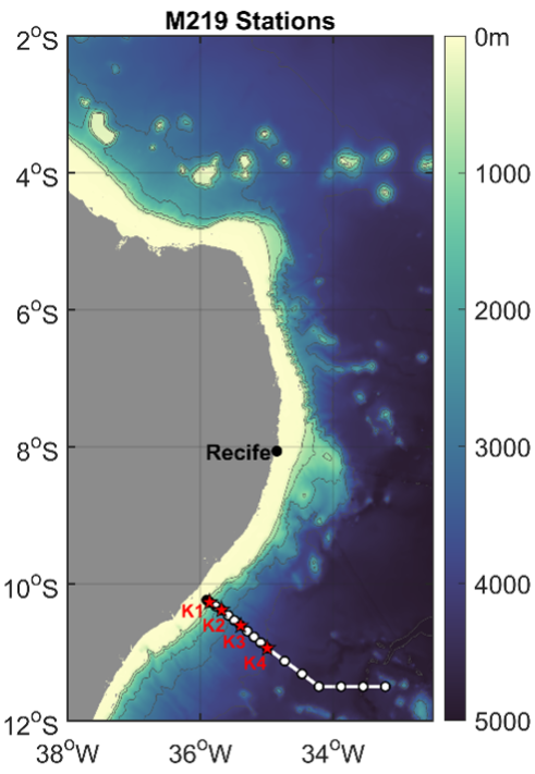
Our first major operations took place off the Brazilian coast at 11°S, where the K1 to K4 moorings form part of a long-term observing system monitoring the western boundary current system and the Atlantic Meridional Overturning Circulation (AMOC). Within just a few days, the four deep-sea moorings were successfully recovered, assessed, serviced, and redeployed.
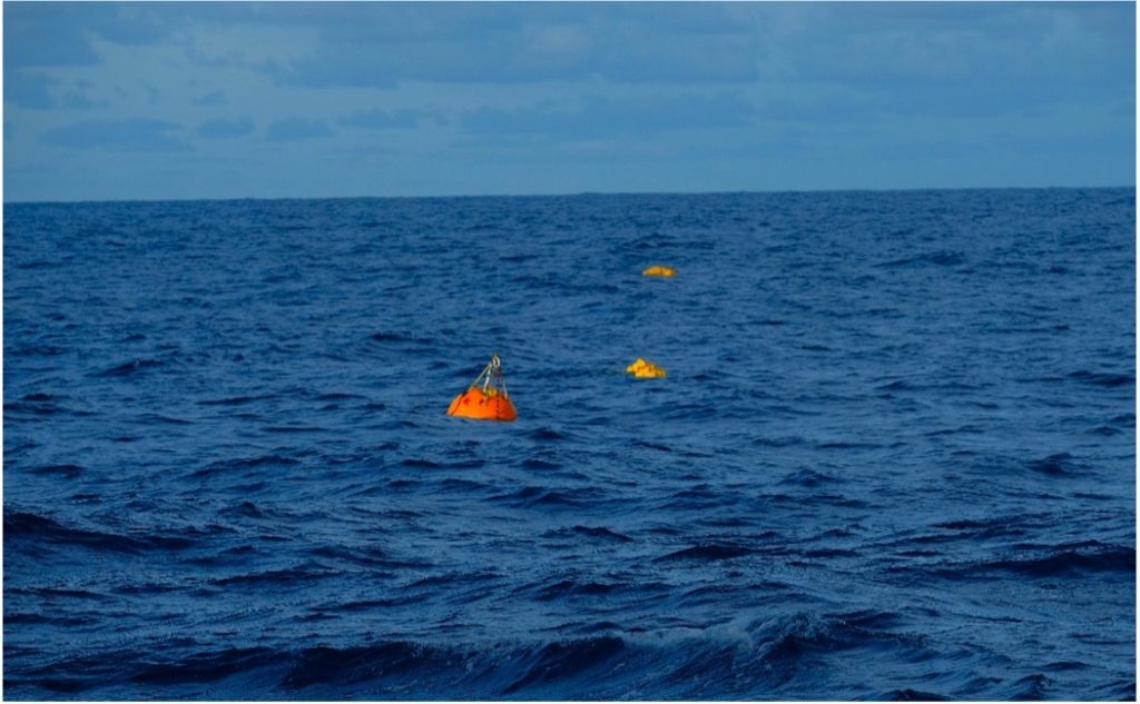
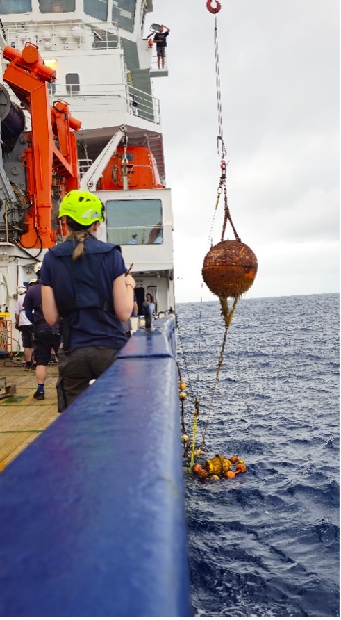
Every recovery felt a bit like opening a treasure chest. After spending a year or more beneath the ocean surface, these instruments returned carrying an invaluable record of currents, temperature, salinity, oxygen, and other key ocean properties. It was incredibly rewarding to see how well they had performed. Nearly all instruments operated successfully throughout the entire deployment period, delivering high-quality datasets with remarkably few gaps.
From Brazil, we continued north to the equator at 23°W, home to another key long-term mooring at exactly 0°N. Since 2006, this mooring has been monitoring the Equatorial Undercurrent and the deep equatorial circulation from the surface to nearly 4,000 m depth. Its successful recovery and redeployment mean that this unique 20-year time series will continue, helping us better understand how the tropical Atlantic influences climate, oxygen and nutrient transport, and marine ecosystems across the basin.
Our final mooring destination brought us to the Cape Verde Ocean Observatory (CVOO), one of the flagship long-term ocean observatories in the eastern tropical Atlantic. Here, physical, biogeochemical, and ecological observations come together to track how the ocean stores heat and carbon and how marine ecosystems respond to environmental change. Like the moorings at 11°S and the equator, the value of CVOO lies not in a single measurement, but in the continuity of the multi-decadal record.
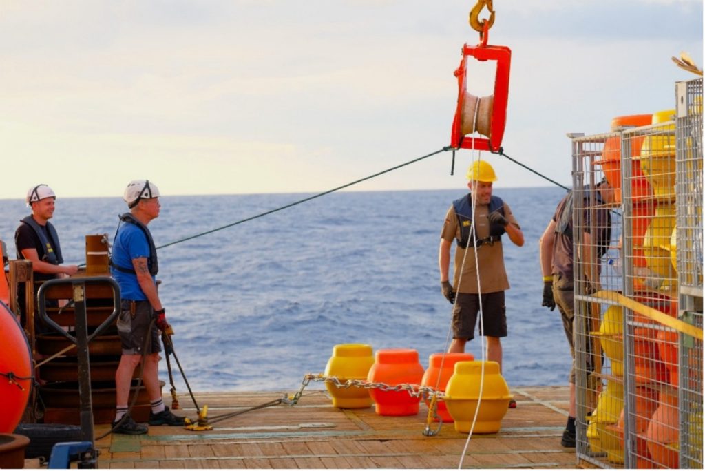
For me, one of the most memorable aspects was seeing how many people contributed to the success of the mooring operations. Careful planning laid the foundation, while having a dedicated person keeping track of every step ensured that everything ran smoothly (kudos to Anna Christina Hans, aka Tina!). On deck, crew, technicians, and scientists worked together like a well-oiled machine, stepping in where needed and solving problems on the fly.
The teamwork extended all the way back home to GEOMAR. Thanks to Rebecca Hummels’ mooring toolbox, data from several instruments could already be processed and checked while parts of the moorings were still in the water, providing an early look at the quality of the observations. On top of that, mooring experts were available around the clock to provide information, advice, and troubleshooting whenever needed. I believe the high success rate of the recoveries and redeployments is a testament to the experience, teamwork, and dedication of everyone involved.
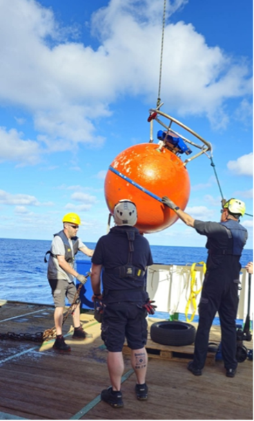
With the major milestone of the successful mooring work behind us, another exciting operation was still ahead. Waiting in Mindelo was a brand-new surface buoy, ready to begin its own contribution to these invaluable long-term observations. Stay tuned to learn more about that deployment in a future blog post.
Keeping the Record Alive: Long-Term Ocean Observations in the Tropical Atlantic

-
Greenhouse Gases10 months ago
Guest post: Why China is still building new coal – and when it might stop
-
Climate Change10 months ago
Guest post: Why China is still building new coal – and when it might stop
-

 Greenhouse Gases2 years ago
嘉宾来稿:满足中国增长的用电需求 光伏加储能“比新建煤电更实惠”
-

 Climate Change2 years ago
嘉宾来稿:满足中国增长的用电需求 光伏加储能“比新建煤电更实惠”
-
Climate Change2 years ago
Bill Discounting Climate Change in Florida’s Energy Policy Awaits DeSantis’ Approval
-

 Renewable Energy8 months ago
Sending Progressive Philanthropist George Soros to Prison?
-

 Carbon Footprint2 years ago
US SEC’s Climate Disclosure Rules Spur Renewed Interest in Carbon Credits
-
Greenhouse Gases11 months ago
嘉宾来稿:探究火山喷发如何影响气候预测