

By Qi-Fan Wu (Niels Bohr Institutet, University of Copenhagen)
During our journey, we saw many beautiful cloud patterns while looking outside the METEOR! Even though people do not always pay attention to them, clouds are among the most visible elements of the sky and naturally form part of our everyday background. And when we sailed away from the coastal region of Recife to the open ocean, the sky seemed to open up, allowing clouds to reveal their full variety and structure.
In climate modelling, clouds are one of the biggest sources of uncertainty. There is a famous saying in mathematics: “Mathematics is the queen of the sciences, number theory is the crown of mathematics, and the Goldbach Conjecture is the pearl on the crown.” The same idea can be applied to the study of clouds in Earth science. There is still no general macroscopic theory of clouds. Cloud physics is an absolutely fascinating topic, as it combines turbulence, stochastic processes, chemicals in the air, multiscale interactions within the Earth–atmosphere system, and a close connection to our daily weather.
In this blog entry, we would like to share some lovely photos of cloud patterns that we took on METEOR. Instead of serious systematic investigations, we focus on the basic cloud physics behind some typical cloud phenomena shown in these photos. These examples might provide something interesting to think about during our leisure time, even after returning to land. If nature is an artist, clouds are among its finest masterpieces, shaped by physical laws and stochastic processes.
What are clouds, and what is inside them? Clouds are made of many liquid water droplets and ice crystals inside the boundaries of the cloud. They are mostly air, with the many particles dispersed widely and more or less randomly throughout the cloud interiors [a]. The individual particles that make up a cloud are very, very small and not generally visible to the human eye.
When we look up from our research vessel METEOR and observe clouds, we first see their macroscopic structure: their overall shape, height, thickness, and organization across the sky. Broad, layered clouds often form through slow, large-scale ascent, while towering clouds with visible turrets reflect rapid rising motion in smaller air parcels. These visible forms are continuously shaped by moisture supply, cooling, turbulence, mixing with drier air, and precipitation, linking the large-scale atmospheric flow to the clouds we observe [a,b].
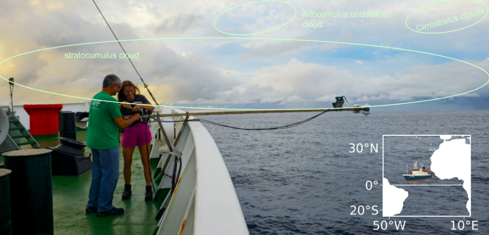
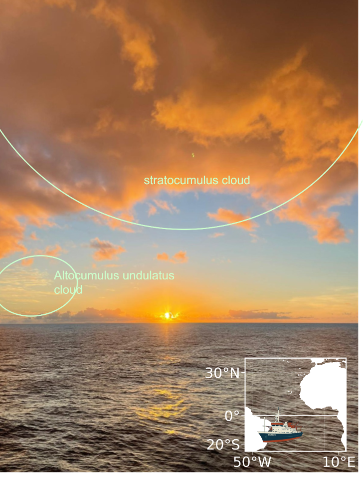
After leaving Recife, we entered a region typically influenced by the southeast trade winds of the tropical South Atlantic, where a vertically layered atmosphere, warm ocean conditions, and wind-driven mixing often promote a turbulent marine boundary layer. In Figure 1, the sky shows a layered cloudscape ranging from thin, high cirrostratus and altocumulus clouds to low cumulus and towering cumulonimbus clouds. These different forms reflect how the atmosphere organizes moisture, cooling, and vertical motion: broad layers are associated with gradual ascent, while the rising turrets of cumulus and cumulonimbus reveal stronger localized updrafts. Together, they illustrate the visible macroscopic structure of clouds, shaped by atmospheric motion and the microphysical processes occurring within them.
It should be noted that, in general, atmospheric temperature in the troposphere decreases with increasing altitude. Over the subtropical oceans, however, this is not the case. A relatively thin temperature-inversion layer lies above the subtropical marine boundary layer, within which temperature increases with height and the atmosphere is highly stable (Figure 2). Cloud occurrence above the marine boundary layer is relatively low in this region. The base of the trade-wind inversion is typically located at an altitude of approximately 1–2 km, separating the moist lower layer from the dry free troposphere [c].
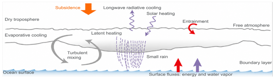
This large-scale thermodynamic structure provides the environmental conditions under which clouds form and evolve. At the microscopic scale, however, clouds consist of particles: liquid water droplets, ice crystals, or a mixture of both. Clouds composed entirely of liquid droplets are commonly referred to as “warm clouds”, whereas clouds containing ice particles are classified as “cold clouds”. When liquid droplets and ice crystals coexist, the cloud is described as a mixed-phase cloud. However, the distinction between “warm” and “cold” clouds hinge on the phase of the particles, not on the temperature. The warm/cold distinction depends on the microphysical phase of the particles inside the cloud, which a normal naked eye observation cannot resolve.
Warm clouds consist of liquid water droplets spanning a range of sizes, from small haze droplets and cloud condensation nuclei to cloud droplets, drizzle drops, and raindrops (Figure 3). Cloud droplets typically form when water vapour condenses onto cloud condensation nuclei. Rainfall develops when some droplets grow much larger: larger droplets fall faster, collide with smaller droplets, and collect them. As a result, many small cloud droplets can combine to form fewer, larger drizzle drops and eventually raindrops [a]. This process approximately conserves the total liquid-water mass within the cloud, while transferring water from numerous small droplets to a much smaller number of large drops that are heavy enough to fall as rain.
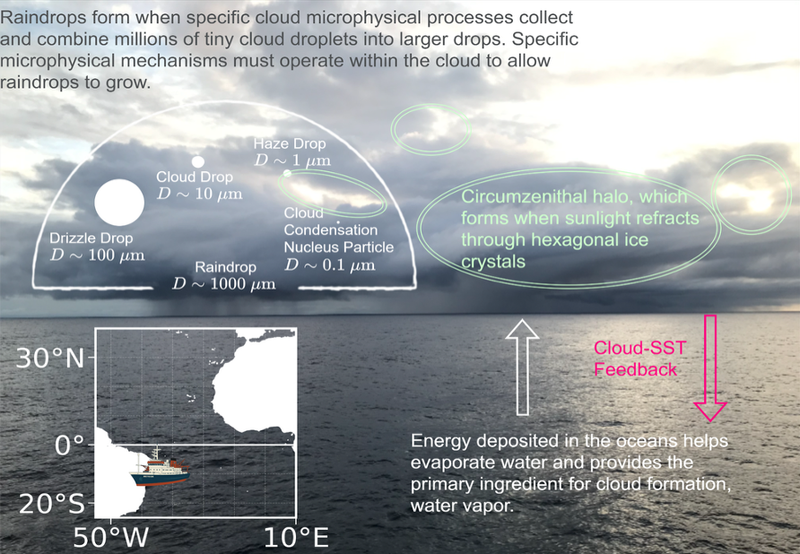
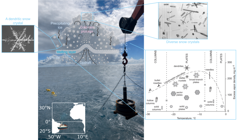
Cold clouds contain ice particles, either alone or together with supercooled liquid water droplets [a]. Unlike liquid droplets, which are nearly spherical because of surface tension, ice particles can develop a wide range of crystalline shapes, including plates, columns, needles, dendrites, and aggregates (Figure 4). Their shape depends mainly on temperature and ice supersaturation during growth by water-vapour deposition. As ice crystals become large enough to fall, they may collide and stick together to form snow aggregates, or collect supercooled droplets that freeze on contact, a process known as riming. The regular hexagonal structure of ice crystals can also produce optical phenomena such as halos, which form when sunlight is refracted or reflected by suitably oriented ice crystals in high-level clouds as shown in Figure 3. In mixed-phase clouds, uplift supports the growth of ice crystals at the expense of supercooled droplets. Once sufficiently large, the ice precipitates and may melt into rain or drizzle while falling through the melting layer (Figure 3).
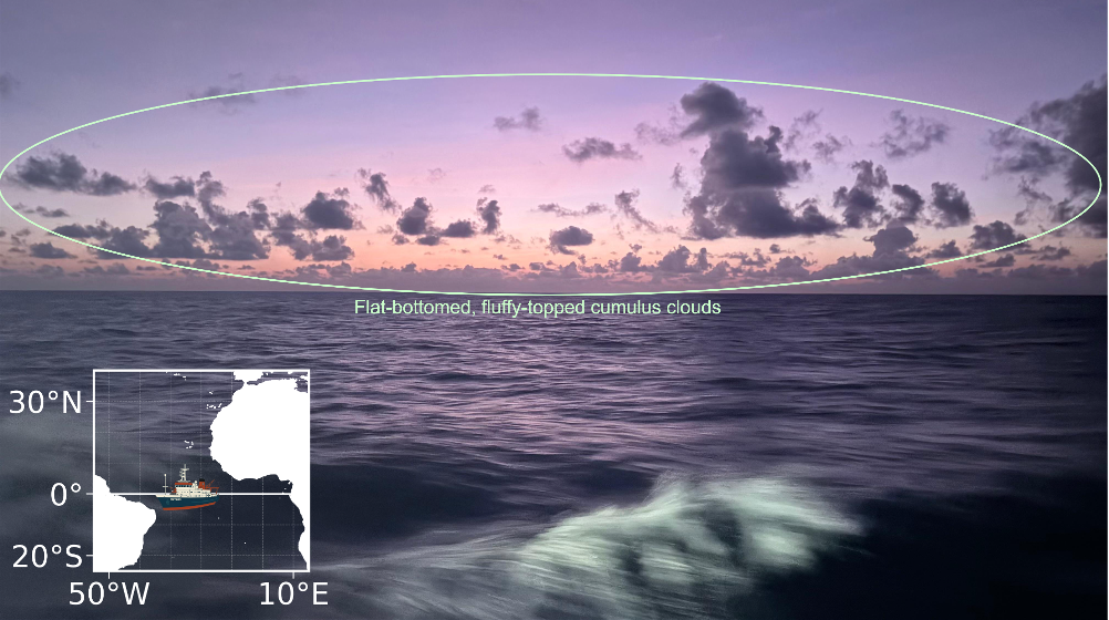
When we approached the equator, we saw many cumulus clouds with remarkably flat bases, marking the lifting condensation level where warm, moist air rising from the ocean cooled to its dew point and condensed into droplets. Similar temperature/humidity across an area leads to clouds sharing flat bases. Their uneven, towering tops reflected continued turbulence and convection above this level, revealing the active vertical mixing of the tropical atmosphere (Figure 5). As moist tropical air rises toward the cold-point tropopause, it encounters extremely low temperatures. When an air mass reaches a local temperature minimum, water vapour can freeze into very thin cirrus clouds (Figure 6).
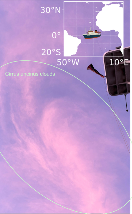
After crossing the equator, we entered the Intertropical Convergence Zone (ITCZ), a band of heavy rainfall extending across the tropical Atlantic. Cloud organization within and around the ITCZ varies markedly from day to day. Extensive low-level stratocumulus clouds can also occur in the surrounding region, acting like a blanket that reduces the amount of incoming solar radiation reaching the ocean surface (Figure 7).
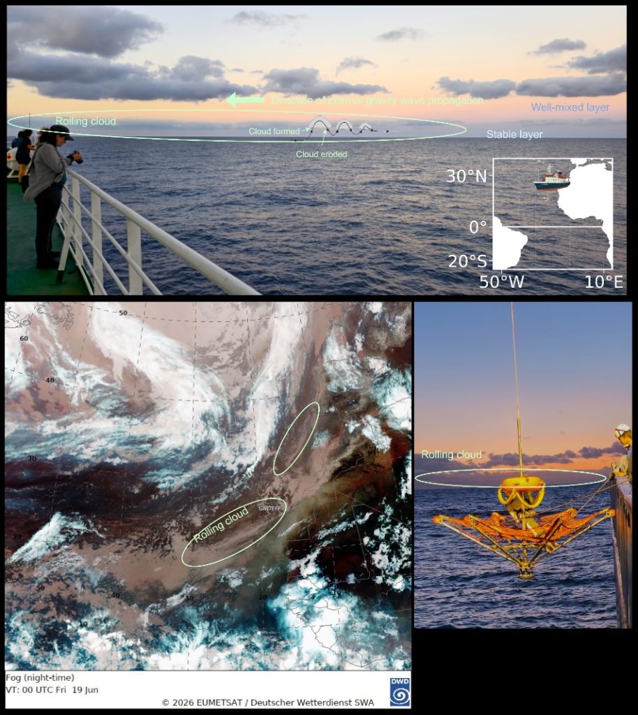
As we continued northward on our way home, we moved closer to the continent and witnessed some spectacular roll clouds, a very rare meteorological phenomenon. This type of cloud is known as “Morning Glory,” although evening land breezes can also produce roll clouds. The roll cloud is not attached to other clouds. associated with a solitary wave, a wave that has a single crest and moves without changing speed or shape.
As we were relatively close to the shoreline of West Africa, these roll clouds may have been produced by internal gravity waves propagating along a stable marine boundary layer [d]. The collision or sudden advance of a sea breeze or cold front can disturb the stable air layer near the surface, generating an atmospheric bore (a train of internal gravity waves). Such waves consist of alternating regions of upward and downward motion. Along the crest of the wave, moist air is lifted and cools to saturation, forming clouds, while behind the crest the air descends and warms, causing the cloud to evaporate. Because this cycle of ascent and descent extends along a long line of low-level convergence, cloud is continuously generated at the leading edge and dissipated at the trailing edge, maintaining a long, coherent band (Figure 8).
I think observing and thinking about clouds can be a nice hobby for enjoying the beauty of nature. Cloud processes are stochastic because nucleation and droplet collection do not occur at exactly the same time for every particle, even under the same environmental conditions [a]. Instead, freezing, condensation, and coalescence depend on chance microscopic events, so only some droplets become “lucky” and grow or freeze earlier than others. Perhaps cloud viewing could also give us good food for thought. After all, many cloud-related problems in climate modeling remain among the most beautiful mysteries in climate science.
Enjoy ~
References:
[a] Lamb D, Verlinde J. Physics and Chemistry of Clouds. Cambridge University Press; 2011.
[b] Levizzani, V., Kidd, C. (2025). Cloud Physics. In: Precipitation. Geophysics and Environmental Physics. Springer, Cham. https://doi.org/10.1007/978-3-031-97096-2_3
[c] Shang-Ping Xie. Subtropical climate: Trade winds and low clouds. In: Coupled Atmosphere-Ocean Dynamics. Elsevier; 2024. p. 139–163. doi:10.1016/B978-0-323-95490-7.00006-0.
[d] The Morning Glory and related phenomena. https://www.meteo.physik.uni-muenchen.de/~roger/AustralianProjects/TheMorningGlory/TheMorningGlory.html

Ocean Acidification
Dr Heidarzadeh’s TV interview with SkyNews on the massive M7.7 Panama earthquake on 9 October 2026
Dr Heidarzadeh’s TV interview with SkyNews on the massive M7.7 Panama earthquake on 9 October 2026. Click here for the full story.

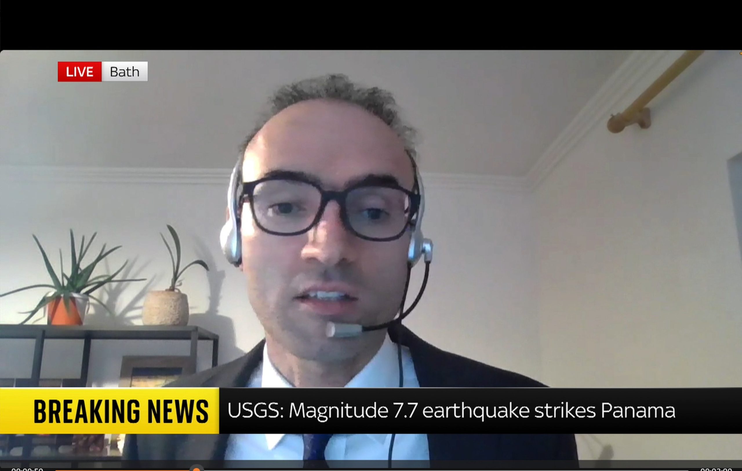
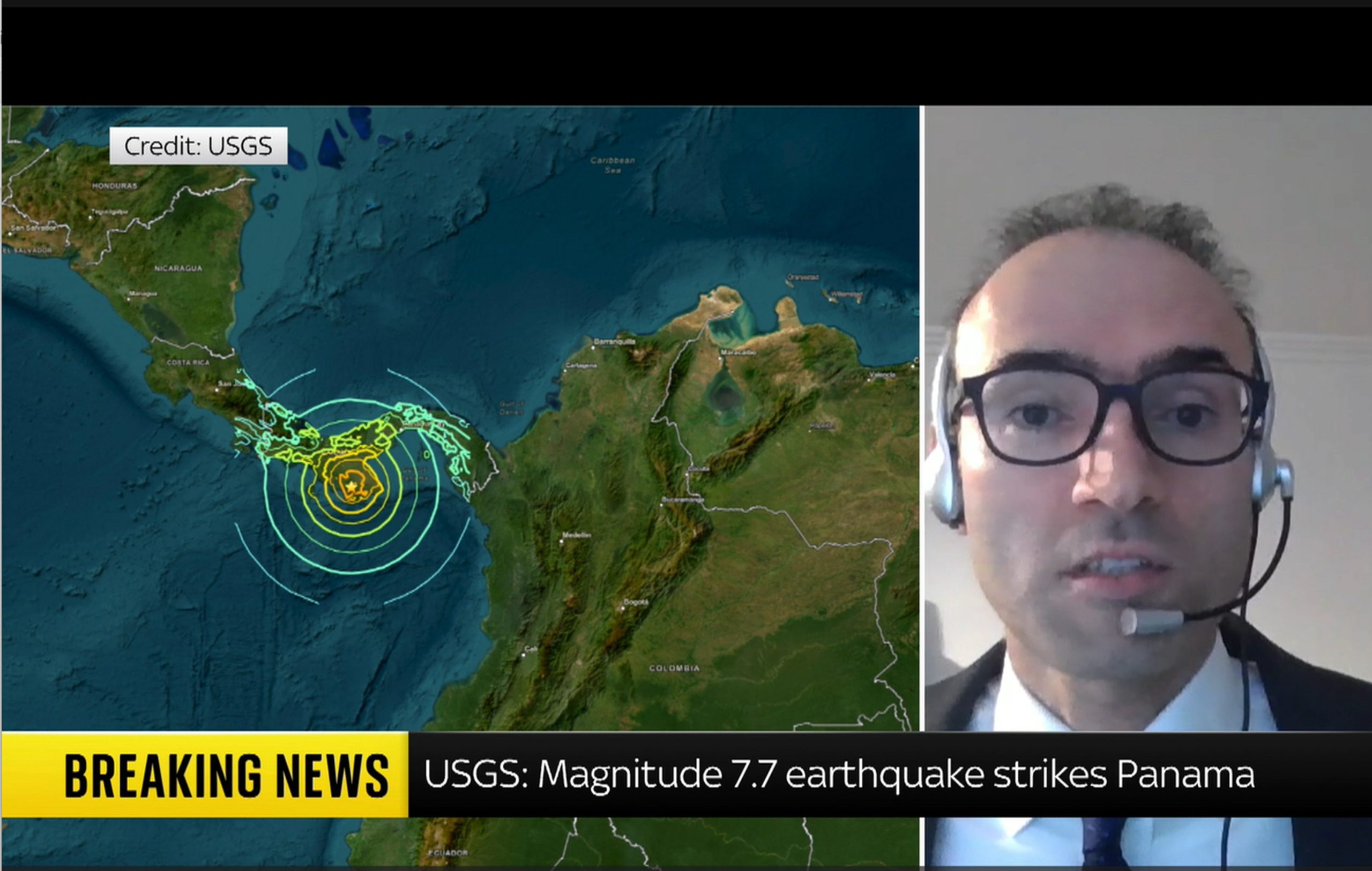
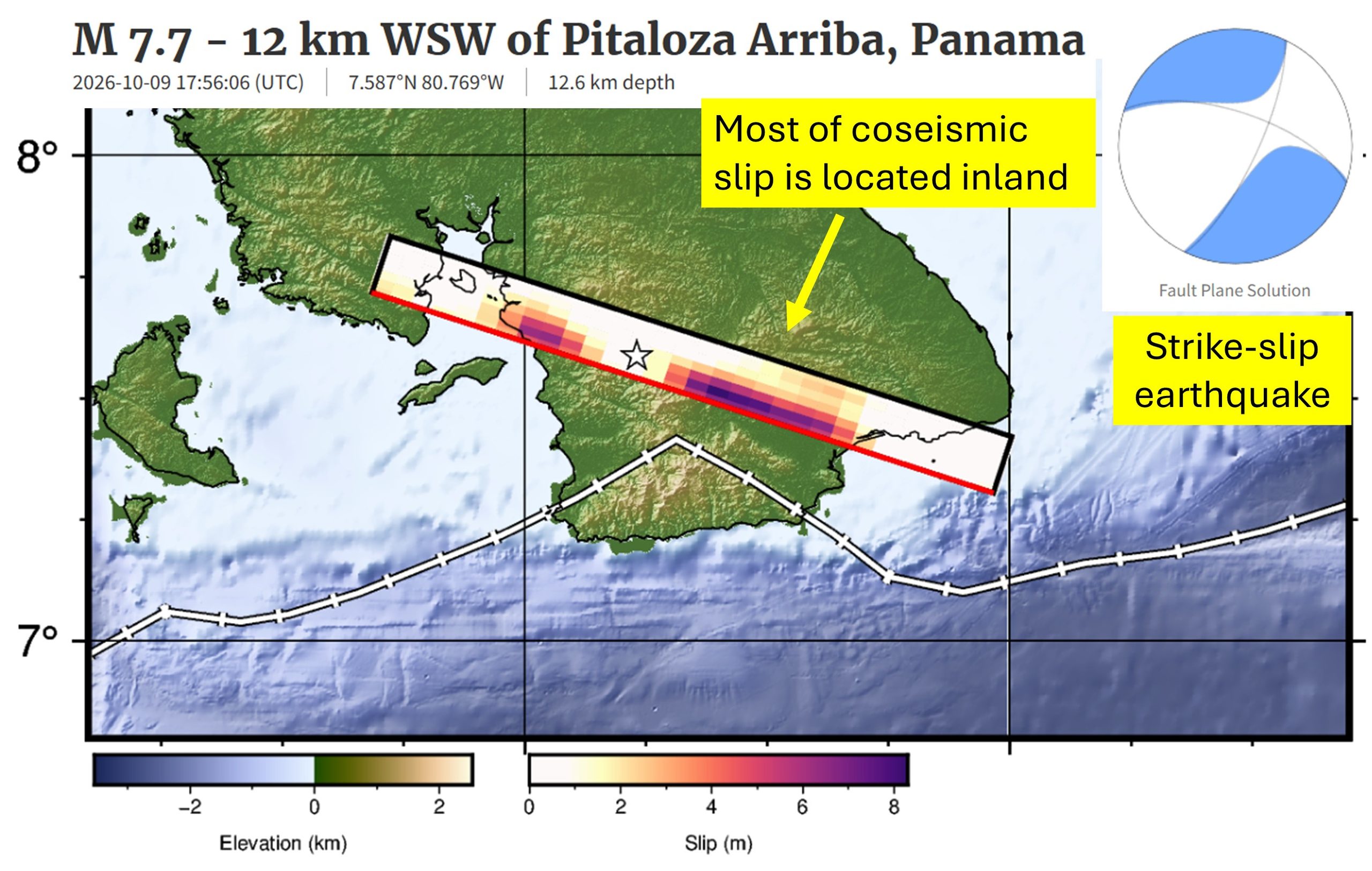
Dr Heidarzadeh’s TV interview with SkyNews on the massive M7.7 Panama earthquake on 9 October 2026
Our ocean is an incredibly vast and mysterious place. And there is no place where that is more evident than the deepest ocean area in the world: the legendary Mariana Trench. Located east of the Philippines, the Mariana Trench lies in the Mariana Archipelago in the western portion of the North Pacific. The greater area of the Mariana Trench Marine National Monument is made up of more than 95,000 square miles of ocean. Beneath these waters lie incredibly complex aggregations of submerged islands and volcanoes … and of course, an astoundingly massive trench.
Dive in with us to have your biggest questions answered about the famed Mariana Trench.
How deep is the Mariana Trench?
The deepest part of the Mariana Trench, known as Challenger Deep, is almost 36,000 feet below the ocean’s surface. For context, Mount Everest is about 29,000 feet above sea level, so the Mariana Trench is about 7,000 feet deeper than Mount Everest is tall. For one more comparison, the RMS Titanic lies at a depth of about 12,500 feet below sea level. The Challenger Deep is in waters nearly three times deeper than this ship’s final resting place.
Due to its enormous size, the Mariana Trench has at times been affectionately nicknamed the Grand Canyon of the ocean. This is certainly a picturesque image, but don’t let the mammoth size of this U.S. national terrestrial park fool you into thinking the Mariana Trench matches its size. The trench’s footprint is estimated to be 120 times larger than the Grand Canyon’s, and to reach the bottom of Challenger Deep, you’d need to descend through almost six Grand Canyons stacked on top of each other before you’d reach the seafloor.
Oh … and did we mention it’s five times wider than it is deep? It’s about 43 miles wide!
What is Challenger Deep, and how long would it take to reach it?
Challenger Deep is the deepest point of the Mariana Trench. Fewer than 30 people have ever journeyed to this area. The trek below the surface is long, dark and time-consuming, and it’s not an expedition considered lightly by scientists and explorers.
The first people to descend into the depths of this area in 1960 were oceanographers Jacques Piccard and Don Walsh, and it took them close to five hours to reach Challenger Deep. Since then, more advanced submersibles have been created, but it still takes two to four hours for modern vessels to reach such depths. For example, explorer and filmmaker James Cameron reached the seafloor in a little more than 2.5 hours in the first documented solo submarine dive to the area, and it took oceanographer Dr. Dawn Wright about four hours in 2022. It is crucial that these submersibles descend slowly and steadily beneath the surface, as the immense water pressure compounds with every mile a submersible descends. Speaking of pressure …
Get Ocean Updates in Your Inbox
Sign up with your email and never miss an update.
What is the water pressure at the bottom of the Mariana Trench?
If you thought the depth of the Mariana Trench was its only jaw-dropping feature, think again. Water pressure is one of the most important factors affecting deep-sea life. In the ocean, pressure increases by one atmosphere for every 33 feet (10 meters) of depth. One atmosphere (a unit of measurement for pressure equivalent to average air pressure at sea level) is equal to about 14.7 pounds per square inch (PSI), which is the approximate standard atmospheric pressure at sea level. If you were to convert atmospheric pressure into weight, one atmosphere is about the weight of a bowling ball. Stay with me, friends.
If a vessel were to dive 2,000 feet below the surface, the pressure would equal that of 60 bowling balls stacked atop every square inch of that submersible. But 60 bowling balls is simply nothing compared to the pressure in the Mariana Trench. The atmospheric pressure at the depths of Challenger Deep is equal to about 16,000 PSI. That pressure is about the same as the weight of an entire full-grown elephant on every square inch of a submersible!
Need a more extreme comparison? If a human were to be placed at the bottom of the Mariana Trench, the pressure would be equal to that of 50 jumbo jets piled on top of a person!
Do any animals live in the Mariana Trench?
The depths of the Mariana Trench come with immense pressure and extreme darkness, but somehow, life finds a way to survive. Organisms that live at an extreme depth, like that of Challenger Deep, have to be highly adapted to low temperatures (typically just above freezing), high pressure and virtually no light at all.
Species found in the depths of the Mariana Trench might look vastly different from animals from other ocean depths because their anatomy has been refined to thrive in harsh conditions. At such great depths, these animals typically depend on chemosynthesis (using nutrient-rich waters being pumped out of hydrothermal vents) or descending detritus (dead matter that has fallen from higher parts of the ocean) for food, such as whale falls. Just a handful of these animals include species of octopuses and squids, sea cucumbers, amphipods, sea jellies, shrimp, sea worms and some wild-looking fish!
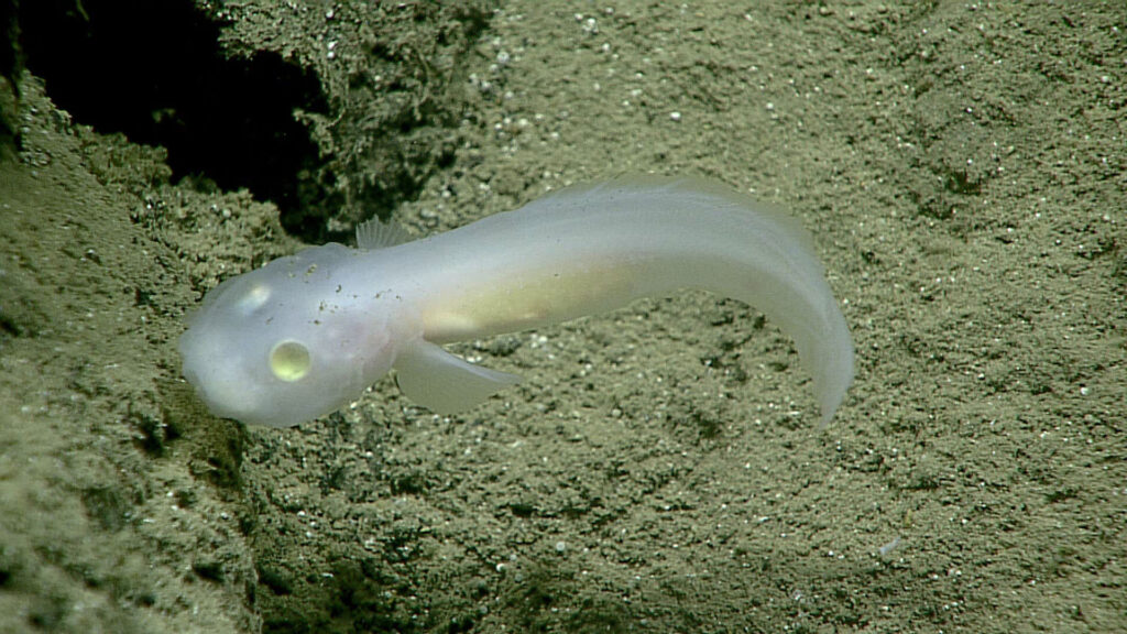
In 2025, more than 7,000 new species were discovered in the Mariana Trench, including the hadal snailfish (Pseudoliparis swirei). This is the deepest-dwelling fish currently known to science. Now, the fish has been dubbed “the Mariana snailfish.”
How was the Mariana Trench formed?
The process by which the Mariana Trench was created is a geologically fascinating one known as subduction. On the Earth’s surface, there are thin plates that cover the planet’s mantle, which is made of molten rock. If two of these plates collide, one pushes down into the Earth’s mantle while the other is pushed over the bottom plate. When this happens, a trench is formed from the drag of the bottom plate. This process can sometimes create incredibly strong earthquakes. The plates that forged the Mariana Trench’s creation are estimated to be up to approximately 180 million years old.
This trench was unknown to scientists until 1875. It was then that a team of explorers on the HMS Challenger measured the depth of the sea by simply lowering a weighted rope into the water. They were baffled when they measured that first portion of the seafloor to be five miles below the surface. And so was born the origin of some of the most daring deep-sea explorations known to mankind to date.
Is the Mariana Trench protected?
The Mariana Trench is in waters off Guam and the Mariana Islands. The region is protected from some human activities under its status as a marine monument. The creation of the Mariana Trench Marine National Monument signified that international, national and local leaders all recognize the importance of protecting this area.
However, just because the region is protected does not mean it’s not vulnerable to modern threats to ocean health. Plastic bags have been spotted in the Mariana Trench during several expeditions, highlighting the far-reaching impact of the marine debris problem. No corner of our ocean is safe from the ever-present threat of plastic pollution. The reality of a changing climate makes the future well-being of wondrous places like the Mariana Trench uncertain. What’s more: More than 70% of the global ocean has yet to be mapped. And what we don’t yet know about, we cannot wisely work to protect.
It’s up to us to work together to defend our ocean, from the sandy shores of our favorite beaches to the deepest, darkest parts of the sea. Together, we can work to protect our ocean as a whole, which ultimately helps protect treasured places like Challenger Deep.
Find out how you can join Ocean Conservancy’s wave of momentum to secure a healthy ocean and a thriving planet, forever and for everyone!
The post The Mysteries of the Mariana Trench appeared first on Ocean Conservancy.