

Seit wir vor fast zwei Wochen Funchal verlassen haben, sind aufregende Planktonlebewesen in die Labore an Bord der RV Merian gekommen. Mehrere Wissenschaftler und Ingenieure aus deutschen, portugiesischen und US-amerikanischen Einrichtungen haben sich im Chemie-, Trocken- und Deckslabor auf dem Hauptdeck niedergelassen, um sich auf Planktonproben und -analysen vorzubereiten. Seitdem hat sich das Hauptdeck in einen lebhaften Basar für Plankton-Kreaturen verwandelt, auf dem mit Pinzetten und Pipetten Proben aus Wasserproben und Planktonnetzen entnommen, in Petrischalen und Bechergläsern konzentriert und bei Bedarf zwischen den Planktologen ausgetauscht werden.


Wir stehen auf, ziehen unsere Arbeitsausrüstung an und machen uns bereit für den ersten CTD-Einsatz an einer der sechs Zielstationen, dem tiefen Plateaugebiet an der Westflanke vor Madeira mit einer maximalen Tiefe von 1500 m. Wir machen uns auf den Weg, um mit 24 an der CTD befestigten Niskin-Flaschen Meerwasser aus verschiedenen Wassertiefen und die darin befindlichen Organismen zu beproben.

Im Mittelpunkt stehen die kleinsten Lebewesen des Planktons, von Bakterien und Phytoplankton (mikroskopisch kleine einzellige Algen) bis hin zu ihren Fressfeinden, dem Zooplankton. Bakterien und einzellige Algen bilden die Basis der marinen Nahrungsnetze und dienen den Räubern im Plankton als optimale Beute. Doch wer frisst wen, wo und wann? Spielen Wassertemperatur, Licht, Salzgehalt und Nährstoffangebot eine Rolle? Sind Beuteart und Beutequalität gleich wichtig? Diese Fragen versuchen wir zu beantworten, insbesondere vor dem Hintergrund der aktuellen Hitzewelle im Nordostatlantik. Ziel ist es, die Saisonalität und Produktivitätsmuster des Planktons zu analysieren, von Bakterien und Phytoplankton an der Basis des Nahrungsnetzes bis hin zu höheren trophischen Ebenen wie Fischlarven und Quallen.
Nach Verlassen des Hafens von Funchal konzentrierten wir uns zunächst auf den Bereich des östlichen Rückens zwischen Madeira und Ilhas Desertas. Hier war die Phytoplankton-Biomasse gleichmäßig in der oberen Wassersäule verteilt, wo die Wassertemperaturen bis in eine Tiefe von 200 Metern konstant bei etwa 20°C liegen. Darunter ist der Lichteinfall auf ein Minimum reduziert und die Phytoplanktonproduktion nimmt ab. Hier verwandeln sich das saftige einzellige Phytoplankton und die Bakterien in Meeresschneepartikel, die nach unten sinken und auf dem Weg in die Tiefe zersetzt werden. Dort übernehmen die Tiere der Tiefsee, die sich von den Schneeflocken, den Resten des reich gedeckten Tisches in der Wassersäule, ernähren.
Im Bereich des Plateaus an der Westflanke Madeiras zeigen die CTD-Profile, dass Phytoplankton in der Oberflächenschicht selten ist, sich aber in einer bestimmten Schicht in etwa 100 Metern Wassertiefe ansammelt. Hier findet die Produktion statt und die Fraßfeinde sind zum Fressen eingeladen. Die CTD mit den Niskin-Flaschen kehrt nach einem tiefen Abstieg bis auf 1500 Meter wieder an die Oberfläche zurück. Nun beginnt der Probennahme-Zirkus, um den Bedarf der Wissenschaftler an Meerwasser aus verschiedenen Tiefen zu decken, um alle erforderlichen Parameter von Salzgehalt, gelöstem Sauerstoff und Nährstoffmessungen bis hin zu Bakterien-, Phytoplankton- und Mikrozooplanktonanalysen zu erfassen. Während einige Parameter nur in den Labors der Heimatinstitutionen analysiert werden können, werden andere Analysen, wie die mikroskopische Zählung und Identifizierung von Phytoplankton und Mikrozooplankton, vor Ort durchgeführt. Dies ermöglicht einen unmittelbaren Einblick in die Struktur der Planktongemeinschaft vor Madeira und fordert und erfreut uns mit der überwältigenden Artenvielfalt, die das subtropische Plankton zu bieten hat.
-

Coccolithophore Scyphosphaera apsteinii -

Radiolarie (Spumellaria) -

Dinoflagellat Tripos sp. -

Ciliat (Strobiliidae)
Während das Phytoplankton in diesen Gewässern in der Regel von kleinen, einzelligen Fraktionen (< 20 Mikrometer) dominiert wird, scheint zu dieser Jahreszeit eine schöne Vielfalt an größeren Kieselalgen zu gedeihen. Das Mikrozooplankton, ihr räuberisches Gegenstück, bereichert die Artenvielfalt zusätzlich und gibt Einblicke in die große Formen- und Funktionsvielfalt an der Basis des Nahrungsnetzes. Die Fraktion der „Mikrograzer“ besteht hauptsächlich aus Ciliaten, Dinoflagellaten, Radiolarien und Copepoden-Nauplien, die als optimale Nahrung für die größeren Zooplanktonarten im Nahrungsnetz dienen.
Wir freuen uns nun auf die verbleibenden Probennahmen während der Fahrt MSM126 und sind schon gespannt auf die bevorstehenden Labor- und Datenanalysen auf der Grundlage der erstaunlichen Probenmenge, die wir während dieser Fahrt sammeln.
Grüße von Bord der MARIA S. MERIAN,
Nicole Aberle-Malzahn and Manfred Kaufmann

Ocean Acidification
Dr Heidarzadeh’s TV interview with SkyNews on the massive M7.7 Panama earthquake on 9 October 2026
Dr Heidarzadeh’s TV interview with SkyNews on the massive M7.7 Panama earthquake on 9 October 2026. Click here for the full story.
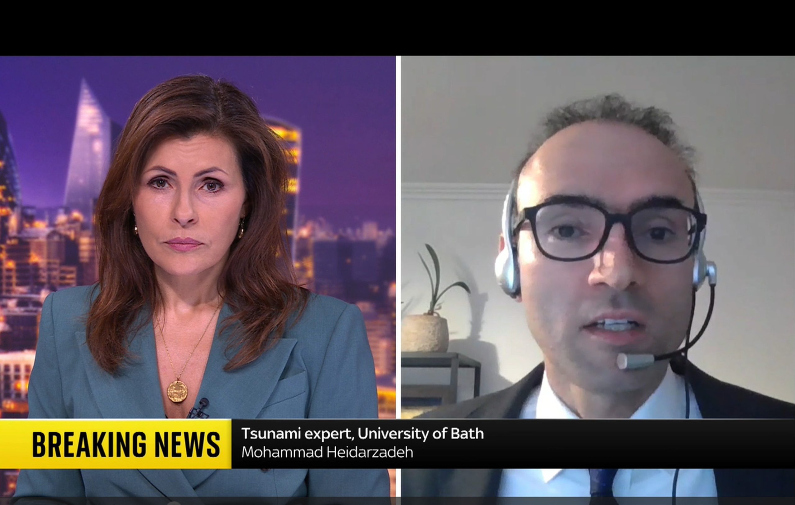
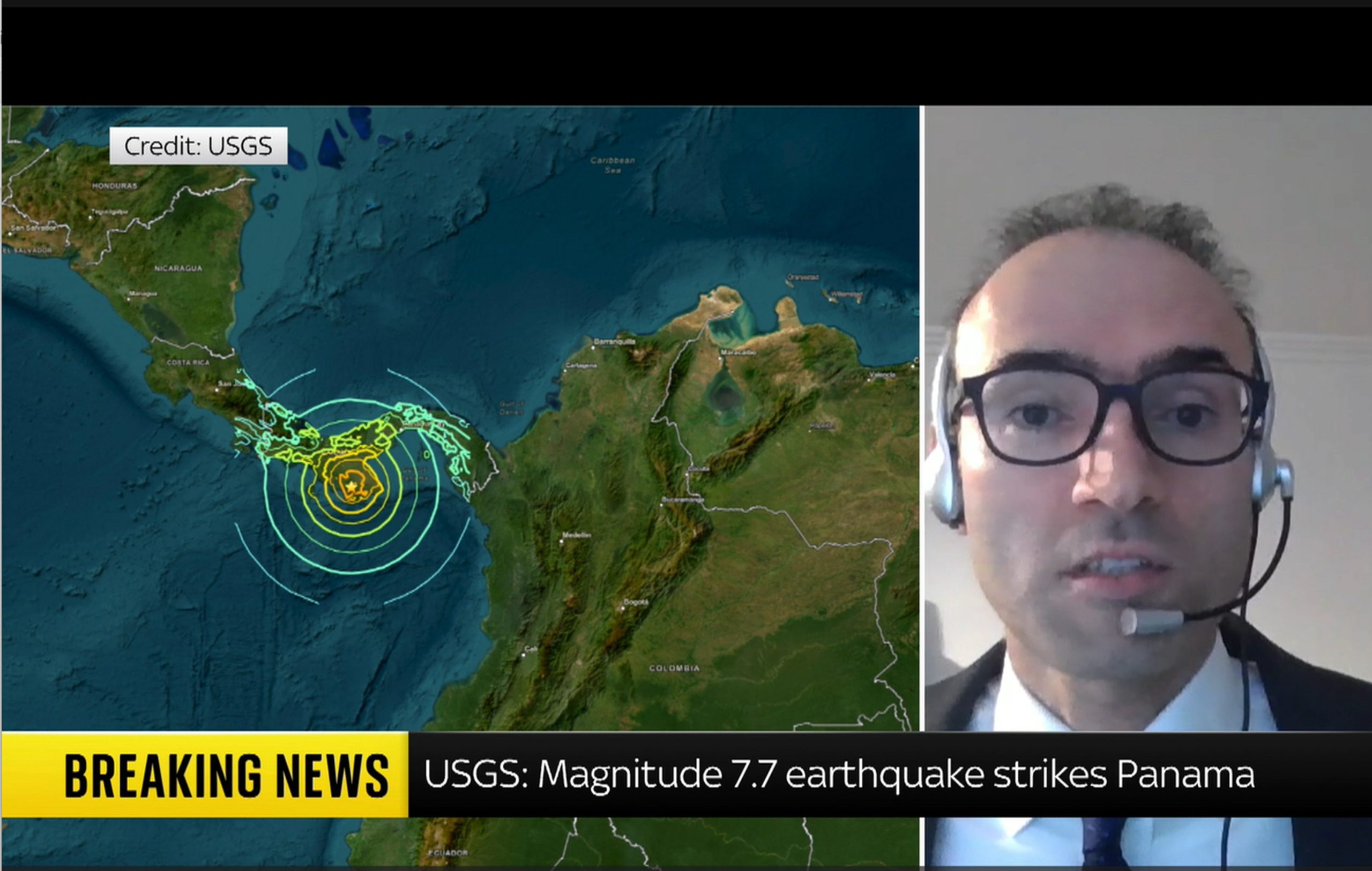
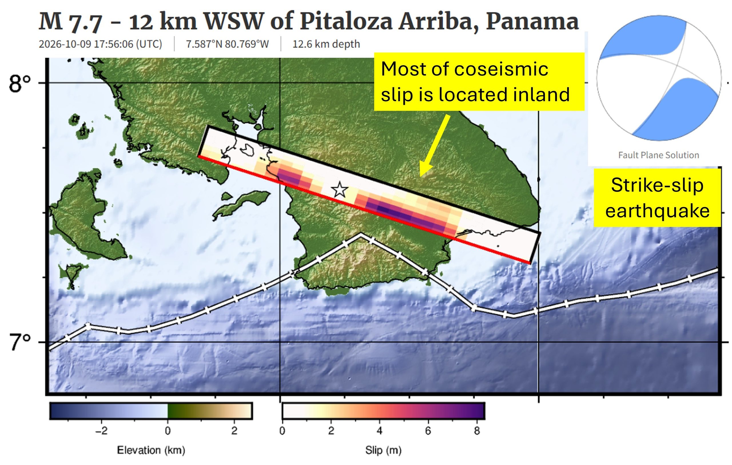
Dr Heidarzadeh’s TV interview with SkyNews on the massive M7.7 Panama earthquake on 9 October 2026
Our ocean is an incredibly vast and mysterious place. And there is no place where that is more evident than the deepest ocean area in the world: the legendary Mariana Trench. Located east of the Philippines, the Mariana Trench lies in the Mariana Archipelago in the western portion of the North Pacific. The greater area of the Mariana Trench Marine National Monument is made up of more than 95,000 square miles of ocean. Beneath these waters lie incredibly complex aggregations of submerged islands and volcanoes … and of course, an astoundingly massive trench.
Dive in with us to have your biggest questions answered about the famed Mariana Trench.
How deep is the Mariana Trench?
The deepest part of the Mariana Trench, known as Challenger Deep, is almost 36,000 feet below the ocean’s surface. For context, Mount Everest is about 29,000 feet above sea level, so the Mariana Trench is about 7,000 feet deeper than Mount Everest is tall. For one more comparison, the RMS Titanic lies at a depth of about 12,500 feet below sea level. The Challenger Deep is in waters nearly three times deeper than this ship’s final resting place.
Due to its enormous size, the Mariana Trench has at times been affectionately nicknamed the Grand Canyon of the ocean. This is certainly a picturesque image, but don’t let the mammoth size of this U.S. national terrestrial park fool you into thinking the Mariana Trench matches its size. The trench’s footprint is estimated to be 120 times larger than the Grand Canyon’s, and to reach the bottom of Challenger Deep, you’d need to descend through almost six Grand Canyons stacked on top of each other before you’d reach the seafloor.
Oh … and did we mention it’s five times wider than it is deep? It’s about 43 miles wide!
What is Challenger Deep, and how long would it take to reach it?
Challenger Deep is the deepest point of the Mariana Trench. Fewer than 30 people have ever journeyed to this area. The trek below the surface is long, dark and time-consuming, and it’s not an expedition considered lightly by scientists and explorers.
The first people to descend into the depths of this area in 1960 were oceanographers Jacques Piccard and Don Walsh, and it took them close to five hours to reach Challenger Deep. Since then, more advanced submersibles have been created, but it still takes two to four hours for modern vessels to reach such depths. For example, explorer and filmmaker James Cameron reached the seafloor in a little more than 2.5 hours in the first documented solo submarine dive to the area, and it took oceanographer Dr. Dawn Wright about four hours in 2022. It is crucial that these submersibles descend slowly and steadily beneath the surface, as the immense water pressure compounds with every mile a submersible descends. Speaking of pressure …
Get Ocean Updates in Your Inbox
Sign up with your email and never miss an update.
What is the water pressure at the bottom of the Mariana Trench?
If you thought the depth of the Mariana Trench was its only jaw-dropping feature, think again. Water pressure is one of the most important factors affecting deep-sea life. In the ocean, pressure increases by one atmosphere for every 33 feet (10 meters) of depth. One atmosphere (a unit of measurement for pressure equivalent to average air pressure at sea level) is equal to about 14.7 pounds per square inch (PSI), which is the approximate standard atmospheric pressure at sea level. If you were to convert atmospheric pressure into weight, one atmosphere is about the weight of a bowling ball. Stay with me, friends.
If a vessel were to dive 2,000 feet below the surface, the pressure would equal that of 60 bowling balls stacked atop every square inch of that submersible. But 60 bowling balls is simply nothing compared to the pressure in the Mariana Trench. The atmospheric pressure at the depths of Challenger Deep is equal to about 16,000 PSI. That pressure is about the same as the weight of an entire full-grown elephant on every square inch of a submersible!
Need a more extreme comparison? If a human were to be placed at the bottom of the Mariana Trench, the pressure would be equal to that of 50 jumbo jets piled on top of a person!
Do any animals live in the Mariana Trench?
The depths of the Mariana Trench come with immense pressure and extreme darkness, but somehow, life finds a way to survive. Organisms that live at an extreme depth, like that of Challenger Deep, have to be highly adapted to low temperatures (typically just above freezing), high pressure and virtually no light at all.
Species found in the depths of the Mariana Trench might look vastly different from animals from other ocean depths because their anatomy has been refined to thrive in harsh conditions. At such great depths, these animals typically depend on chemosynthesis (using nutrient-rich waters being pumped out of hydrothermal vents) or descending detritus (dead matter that has fallen from higher parts of the ocean) for food, such as whale falls. Just a handful of these animals include species of octopuses and squids, sea cucumbers, amphipods, sea jellies, shrimp, sea worms and some wild-looking fish!
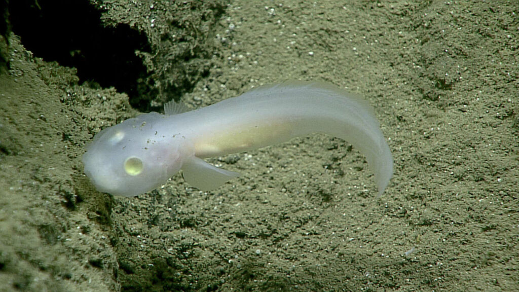
In 2025, more than 7,000 new species were discovered in the Mariana Trench, including the hadal snailfish (Pseudoliparis swirei). This is the deepest-dwelling fish currently known to science. Now, the fish has been dubbed “the Mariana snailfish.”
How was the Mariana Trench formed?
The process by which the Mariana Trench was created is a geologically fascinating one known as subduction. On the Earth’s surface, there are thin plates that cover the planet’s mantle, which is made of molten rock. If two of these plates collide, one pushes down into the Earth’s mantle while the other is pushed over the bottom plate. When this happens, a trench is formed from the drag of the bottom plate. This process can sometimes create incredibly strong earthquakes. The plates that forged the Mariana Trench’s creation are estimated to be up to approximately 180 million years old.
This trench was unknown to scientists until 1875. It was then that a team of explorers on the HMS Challenger measured the depth of the sea by simply lowering a weighted rope into the water. They were baffled when they measured that first portion of the seafloor to be five miles below the surface. And so was born the origin of some of the most daring deep-sea explorations known to mankind to date.
Is the Mariana Trench protected?
The Mariana Trench is in waters off Guam and the Mariana Islands. The region is protected from some human activities under its status as a marine monument. The creation of the Mariana Trench Marine National Monument signified that international, national and local leaders all recognize the importance of protecting this area.
However, just because the region is protected does not mean it’s not vulnerable to modern threats to ocean health. Plastic bags have been spotted in the Mariana Trench during several expeditions, highlighting the far-reaching impact of the marine debris problem. No corner of our ocean is safe from the ever-present threat of plastic pollution. The reality of a changing climate makes the future well-being of wondrous places like the Mariana Trench uncertain. What’s more: More than 70% of the global ocean has yet to be mapped. And what we don’t yet know about, we cannot wisely work to protect.
It’s up to us to work together to defend our ocean, from the sandy shores of our favorite beaches to the deepest, darkest parts of the sea. Together, we can work to protect our ocean as a whole, which ultimately helps protect treasured places like Challenger Deep.
Find out how you can join Ocean Conservancy’s wave of momentum to secure a healthy ocean and a thriving planet, forever and for everyone!
The post The Mysteries of the Mariana Trench appeared first on Ocean Conservancy.
Intro
At the western tip of Luzon, which is the biggest island of the Philippines, lies the small coastal town of Bolinao. Tourists seldom find their way here as it takes around seven hours to get here by bus from Manila. Still, you can spot foreigners walking around every now and then, but they really stand out among the Filipinos. A reason for their presence is often that they study or work at the Bolinao Marine Laboratory (BML), which belongs to the University of the Philippines (UP). It is one of the seven research institutions participating in the GAME project 2026. Every year, GAME brings together Master’s students from all over the world to experience different cultures and conduct globally replicated experiments in marine ecology.
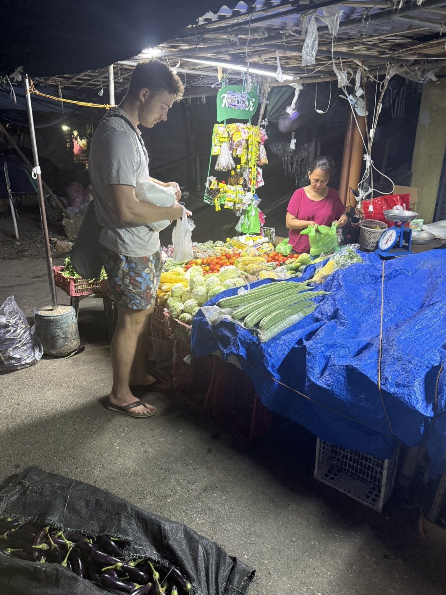
This year’s Team Philippines consists of Jona, a Filipino master student of Marine Biology at the University of the Philippines, and Konstantin, a German student who is enrolled in the Master programme „Ecology and Evolution“ at Freiburg University. As part of GAME 2026, we are currently staying at BML for 6 months to run experiments about the influence of underwater soundscapes on the colonization of marine hardbottoms.
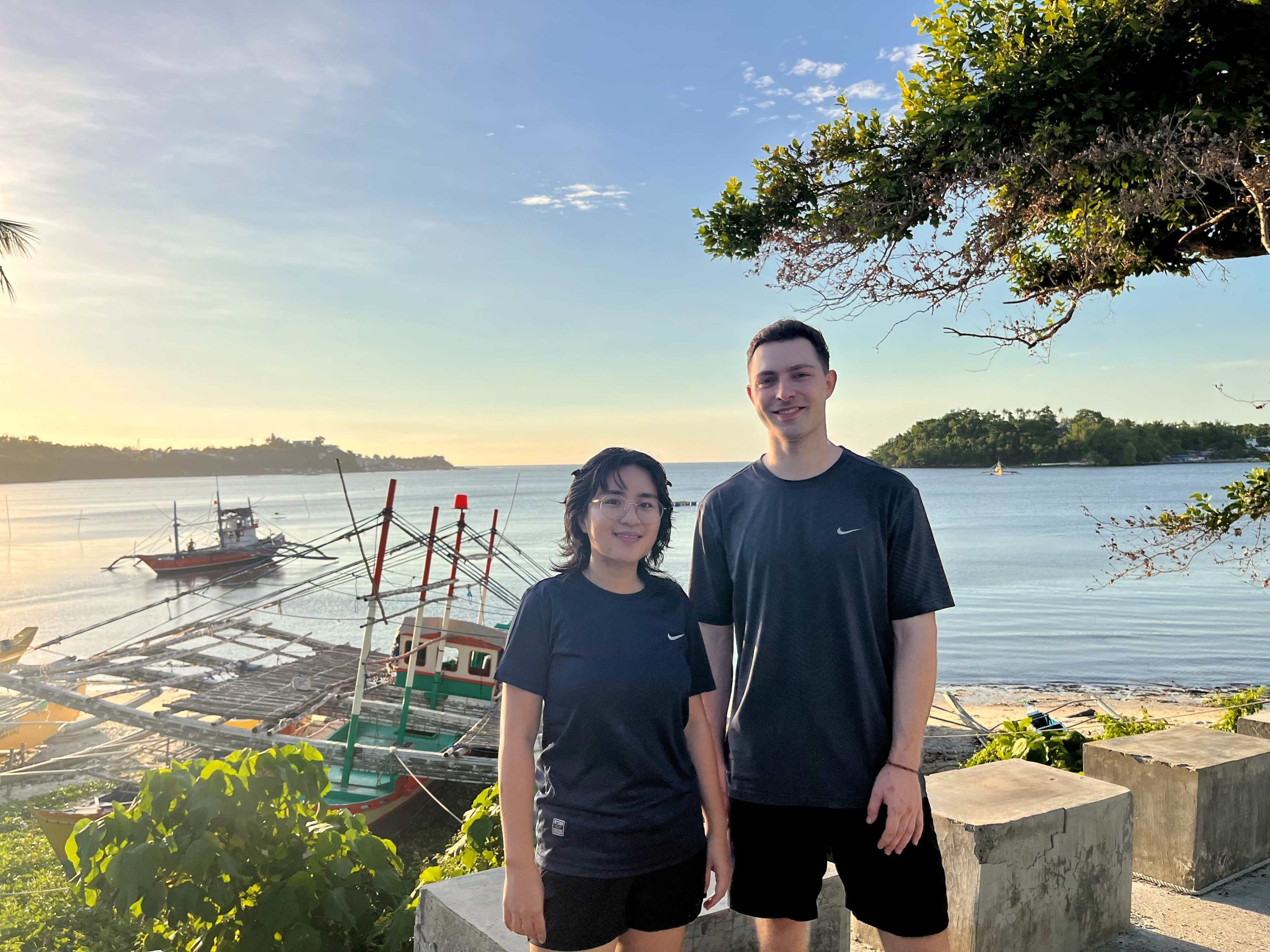
Where are we?
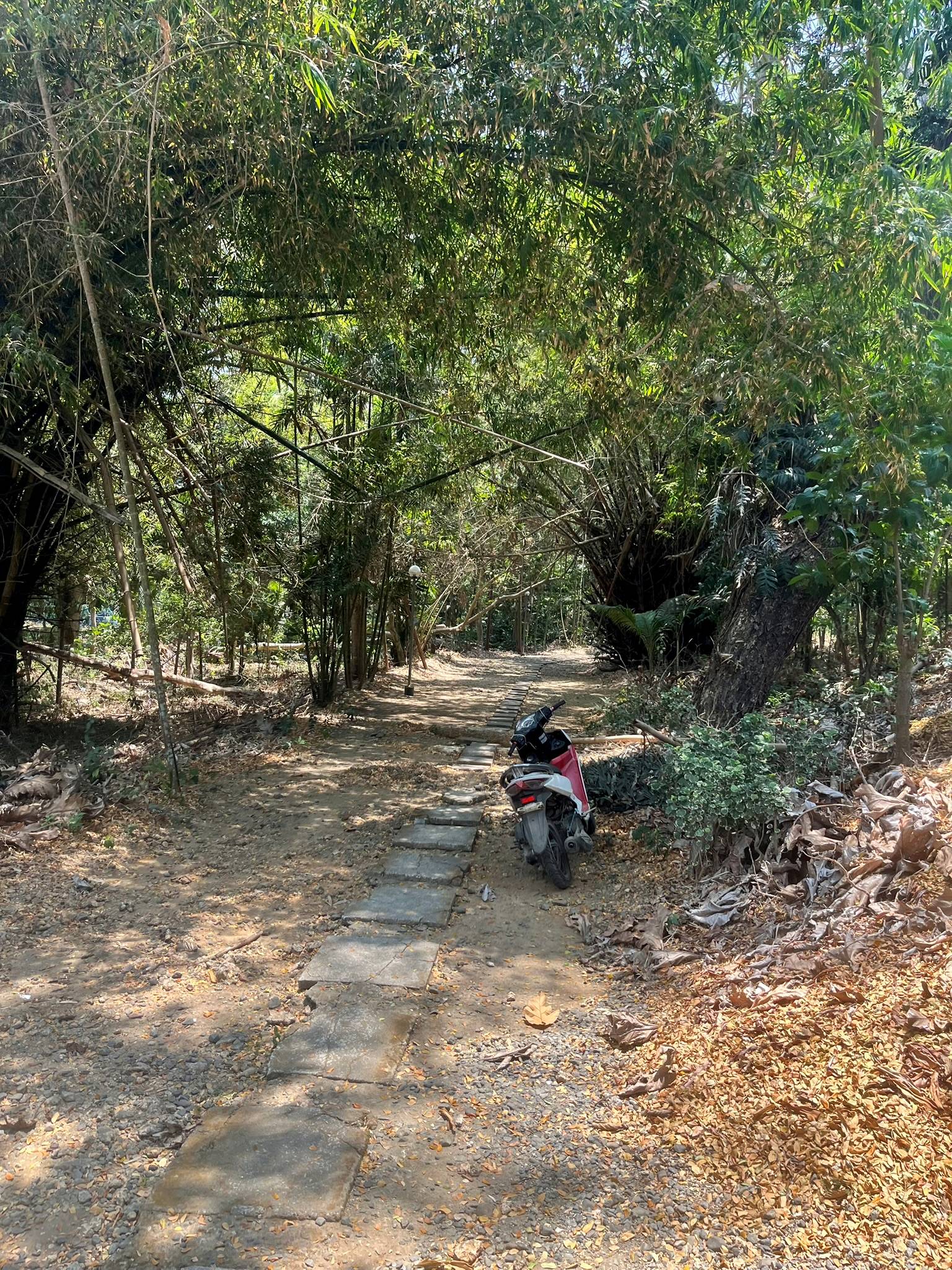
At the BML, we live in a dormitory together with many other students and scientists mostly from the Philippines and a few international interns. At almost any time of the day there is someone in the kitchen to hang out with, eat together, or simply have a chat. It is easy to make friends in this little community. The way to work is just a short walk along a forest path, where we can pick mangos for a snack and spot butterflies, birds, or even wild macaques climbing through the trees. After crossing a street, we reach the institute. But instead of enjoying the cool temperatures of the laboratories, we spend most of our working days outside, doing fieldwork in or near the water.
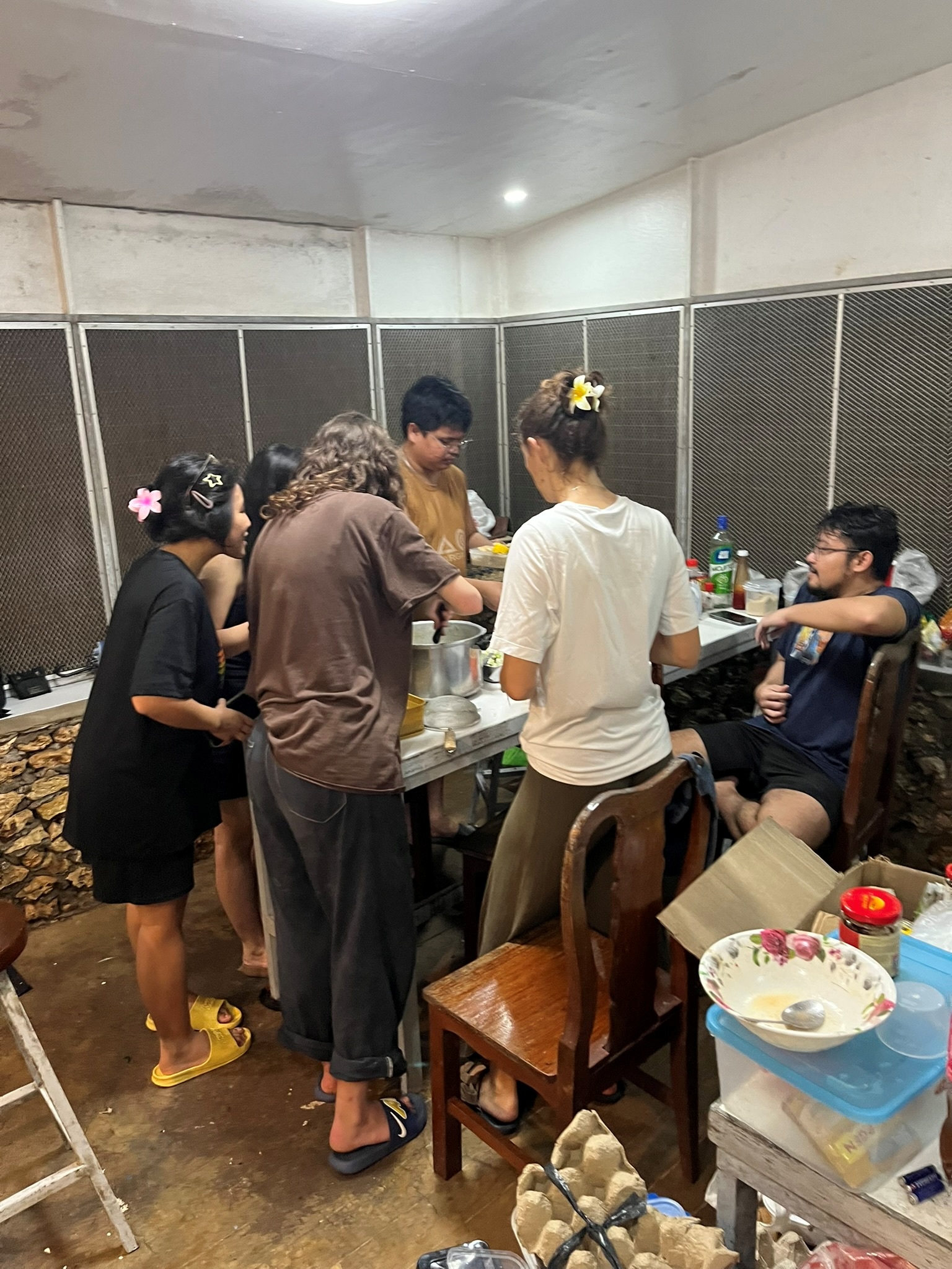
On Fridays, Konstantin experiences real Filipino culture during an almost weekly party at the institute