

The Greenland ice sheet melt season for this year is over, resulting in the 28th year in a row in which Greenland has lost ice.
This has been a spiky year for Greenland – a mix of highs from abundant snow in winter and lows from some very high melt days in summer.
Those spikes of high snowfall delayed the onset of the melt season in June and reduced melt substantially in August. Fresh snow is a brighter white than old glacier ice, so summer snow effectively acted as a shiny protective blanket – just when the high melt season was getting going.
The 2023-24 year, as the year before, had strong melt rates throughout the northern-hemisphere summer, but also above average snowfall during winter and in June. As a result, the balance between accumulated snow and melting ice on Greenland’s surface ended above the 1981-2010 average.
The increase in both melt and snowfall are exactly what scientists expect in a warming climate. But, overall, Greenland has again lost more ice than it gained – even though, as in previous years, Greenland was comparably cool compared to North America and Europe.
High “calving” rates – the breaking off of icebergs at the face of the ice sheet – meant that Greenland lost 80bn tonnes of ice over the 12 months from September 2023 to August 2024. The last year to see a net gain of ice is still 1996.
This marks the 10th year of these annual reviews – see our previous annual analysis for 2023, 2022, 2021, 2020, 2019, 2018, 2017, 2016 and 2015.
Surface melt
Greenland’s annual cycle covers the 12 months from the previous September up to the end of August. Over this period, we calculate the “surface mass budget” (SMB) for the ice sheet.
The SMB is akin to the bank account for the surface of the Greenland ice sheet. It is the balance between gains (from snowfall) and losses (from ice melt and runoff).
As the ice sheet largely gains snow from September, accumulating ice through autumn, winter and into spring, we start the ice budget year on 1 September.
Then, as the year warms up into late spring, the ice sheet begins to lose more ice through surface melt than it gains from fresh snowfall, generally from the mid of June.
This melt season usually continues until the middle or end of August, the end of the surface budget year.
Snowfall is the only way for the ice sheet to gain mass. Therefore, for the size of the ice sheet to remain constant, this snow must outweigh all other ways the ice sheet can lose ice – iceberg calving, melt at the base of the ice sheet and evaporation from the surface.
According to our calculations, the Greenland ice sheet ended the year 2023-24 with an overall SMB of about 367bn tonnes (Gt). This is the 19th highest SMB in a dataset that goes back 44 years, and it is close to the 1981-2010 average of 348 Gt.
The past year’s SMB is illustrated in the maps and charts below, based on data from the Polar Portal. The blue line in the upper chart shows the day-to-day SMB. Large snowfall events become visible as “spikes”. The blue line in the lower chart depicts the accumulated SMB, counted from the beginning of the “mass balance year” on 1 September 2023. In grey, the long-term average and its variability are shown. For comparison, the red line shows the record-low year of 2011-12.
The map shows the geographic spread of SMB gains (blue) and losses (red) for 2023-24, compared to the long-term average. This shows that southern Greenland had a relatively wet year compared to the long-term average, but the north-west and west lost more than usual. The spikes of snow and melt are clear in the graphs on the right.

Heat over Europe and North America, cool over Greenland
While southern Europe sweltered through multiple heatwaves, northern Europe (with the exception of Arctic Scandinavia) had a rather cool and rainy July, followed by a warmer and sunnier late summer. Svalbard also suffered record temperatures and record amounts of glacier loss this year.
And, yet, Greenland was spared these bouts of heat.
As in previous summer seasons, the comparatively wet and cool spells over the Greenland ice sheet were due to “blocking” weather patterns with ridges over North America and Europe and a trough in between over Greenland.
These high-pressure weather systems have a huge impact on weather extremes. Strong persistent blocks over North America and Europe were present in the course of the summer. This resulted in widespread heat near the cores of these high pressure areas and several heavy rainfall events in various European countries in May and June.
In such a blocked flow, the jet stream is shaped like the Greek capital letter Omega (Ω). With the jet stream bulging up to the north over Canada and northern Europe, troughs of low pressure are found at each “foot” of the omega – including over Greenland.
Svalbard was caught in one the opposite part of the omega with high temperatures and warm air directly over the islands, bringing large amounts of ice melt.
This contrast between Greenland on the one side and Svalbard and the eastern part of Canada is also a common pattern and shows how focusing on extremes in one region of the world means missing out on the opposite extreme in a different region.
The maps below show two examples of these recurring circulation patterns from late May/early June and mid-August. The blue shading shows the cool weather over Greenland (in the centre of the map), while the red shading shows the high temperatures over Canada, Europe and Svalbard .

Snow accumulation
However, the surface mass budget is not just about ice melt.
September, October and November all saw above-average snowfall. Then, as in 2022-23, a rather dry period followed in late winter, followed by spikes in snow in March, April and May.
As a result, the accumulated SMB was close to the 1981-2010 average as melting began.
Subsequently, in June, several large snow fall events brought an emergency blanket back to the ice sheet, delaying the start of the “ablation” – or melt – season to 24 June, 11 days later than the 1981-2010 median. (The ablation season is defined as the first day of three days in a row with an SMB below -1Gt.)
The melt area was well above the average for the period of 1981-2010 during most of June, July and August – despite another spike in snow in August.
The left map shows the area of ice melt on 18 July – the day with the maximum melt extent (67%) of this summer (shaded in red). The map on the right shows the situation at the end of the season on 31 August when the ice sheet was well back into the winter pattern.
The charts beneath show the daily extent of melting across the ice sheet as a percentage (blue line), with the 1981-2010 average shown in grey.

The total mass budget
The surface budget is just one component of the “total” mass budget (TMB) of the Greenland ice sheet:
TMB = SMB + MMB + BMB
Here, MMB is the “marine” mass balance, consisting of the breaking off – or “calving” – of icebergs and the melting of the front of glaciers where they meet the warm sea water. BMB is the “basal” mass balance, which refers to ice losses from the base of the ice sheet. This makes a small, but non-zero, contribution to the TMB and mainly consists of frictional effects and the ground heat flux.
The figure below shows how much ice the Greenland ice sheet has lost (red) going back to 1987, which includes the SMB (blue), MMB (green) and BMB (orange).
For 2023-24, the TMB ended with a loss of 80Gt of ice. This means that 2023-24 was the 28th year in a row with a Greenland ice sheet overall mass loss. As the chart shows, Greenland last saw an annual net gain of ice in 1996.

Satellite data
Using data from the GRACE satellites, we can also estimate how much ice Greenland lost – independently from our calculations above.
The distance of these twin satellites changes slightly due to tiny gravity differences caused by mass changes. In addition, we can measure the speed at which ice flows through control points on the ice sheet where we know the thickness and shape of the ice. Thus, we can estimate MMB, the amount of ice being lost by the process of calving and submarine melting.
This data is openly available, allowing us to monitor the whole ice-sheet budget.
The map and graph below show the gain (blue) and loss (red) in the mass of ice. The difference in these mass changes over a glaciological year (September-August) is the TMB of the ice sheet for that particular year.

According to the GRACE satellite data, most of the ice loss over 2023-24 occurred along the edge of the ice sheet, in particular along the west coast. This is backed up both by PROMICE observations and model data. In the interior of Greenland, a small increase in ice mass is found, as there is usually little or no snow melt in this region.
The graph illustrates the month-by-month development in changes of mass measured in gigatonnes, relative to April 2002. The left axis on the graph shows how this ice mass loss translates into a sea level rise contribution, where 100Gt corresponds to 0.28mm of global sea level rise.
Our calculations and the GRACE satellite data are entirely independent ways of estimating Greenland’s TMB, yet the results are quite closely aligned. From April 2002 to May 2024, the ice sheet losses amounted to 4,756Gt (calculations) and 4,911Gt (satellites) of ice.
As 1Gt of water is equivalent to a cube of 1 km by 1 km by 1 km, 360 of these cubes is equivalent to 1mm of sea level rise averaged around the whole globe.
This means that, since 2002, the Greenland ice sheet alone has contributed around 14mm to global average sea level rise.



The post Guest post: How the Greenland ice sheet fared in 2024 appeared first on Carbon Brief.

Drought and heatwaves occurring together – known as “compound” events – have “surged” across the world since the early 2000s, a new study shows.
Compound drought and heat events (CDHEs) can have devastating effects, creating the ideal conditions for intense wildfires, such as Australia’s “Black Summer” of 2019-20 where bushfires burned 24m hectares and killed 33 people.
The research, published in Science Advances, finds that the increase in CDHEs is predominantly being driven by events that start with a heatwave.
The global area affected by such “heatwave-led” compound events has more than doubled between 1980-2001 and 2002-23, the study says.
The rapid increase in these events over the last 23 years cannot be explained solely by global warming, the authors note.
Since the late 1990s, feedbacks between the land and the atmosphere have become stronger, making heatwaves more likely to trigger drought conditions, they explain.
One of the study authors tells Carbon Brief that societies must pay greater attention to compound events, which can “cause severe impacts on ecosystems, agriculture and society”.
Compound events
CDHEs are extreme weather events where drought and heatwave conditions occur simultaneously – or shortly after each other – in the same region.
These events are often triggered by large-scale weather patterns, such as “blocking” highs, which can produce “prolonged” hot and dry conditions, according to the study.
Prof Sang-Wook Yeh is one of the study authors and a professor at the Ewha Womans University in South Korea. He tells Carbon Brief:
“When heatwaves and droughts occur together, the two hazards reinforce each other through land-atmosphere interactions. This amplifies surface heating and soil moisture deficits, making compound events more intense and damaging than single hazards.”
CDHEs can begin with either a heatwave or a drought.
The sequence of these extremes is important, the study says, as they have different drivers and impacts.
For example, in a CDHE where the heatwave was the precursor, increased direct sunshine causes more moisture loss from soils and plants, leading to a drought.
Conversely, in an event where the drought was the precursor, the lack of soil moisture means that less of the sun’s energy goes into evaporation and more goes into warming the Earth’s surface. This produces favourable conditions for heatwaves.
The study shows that the majority of CDHEs globally start out as a drought.
In recent years, there has been increasing focus on these events due to the devastating impact they have on agriculture, ecosystems and public health.
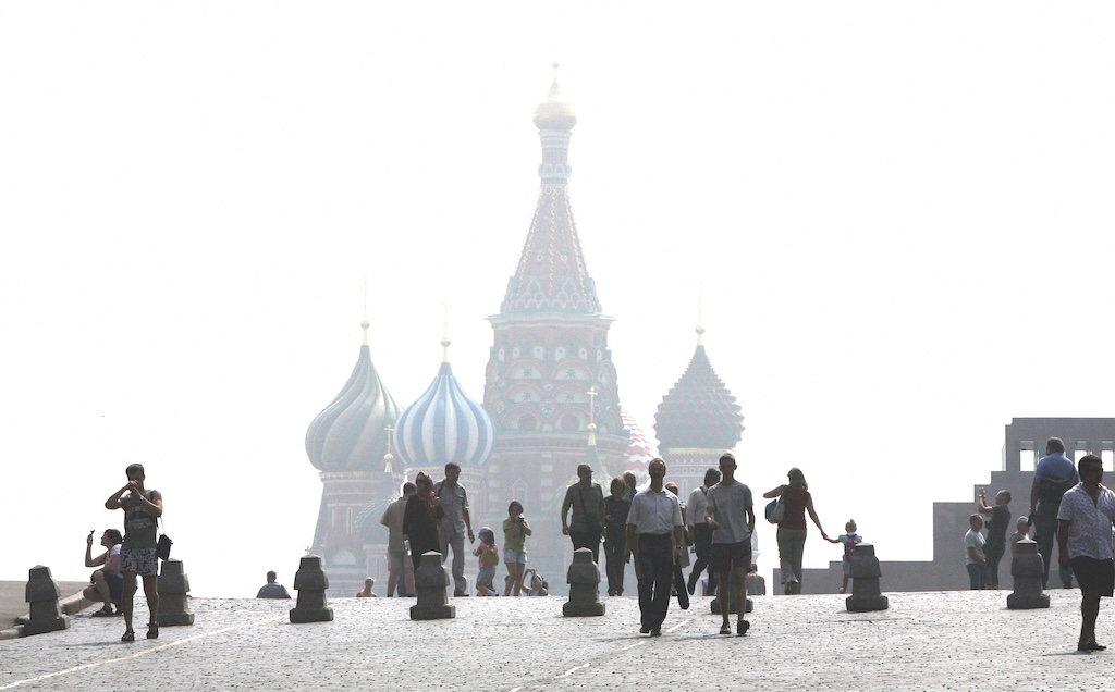
In Russia in the summer of 2010, a compound drought-heatwave event – and the associated wildfires – caused the death of nearly 55,000 people, the study notes.
The record-breaking Pacific north-west “heat dome” in 2021 triggered extreme drought conditions that caused “significant declines” in wheat yields, as well as in barley, canola and fruit production in British Columbia and Alberta, Canada, says the study.
Increasing events
To assess how CDHEs are changing, the researchers use daily reanalysis data to identify droughts and heatwaves events. (Reanalysis data combines past observations with climate models to create a historical climate record.) Then, using an algorithm, they analyse how these events overlap in both time and space.
The study covers the period from 1980 to 2023 and the world’s land surface, excluding polar regions where CDHEs are rare.
The research finds that the area of land affected by CDHEs has “increased substantially” since the early 2000s.
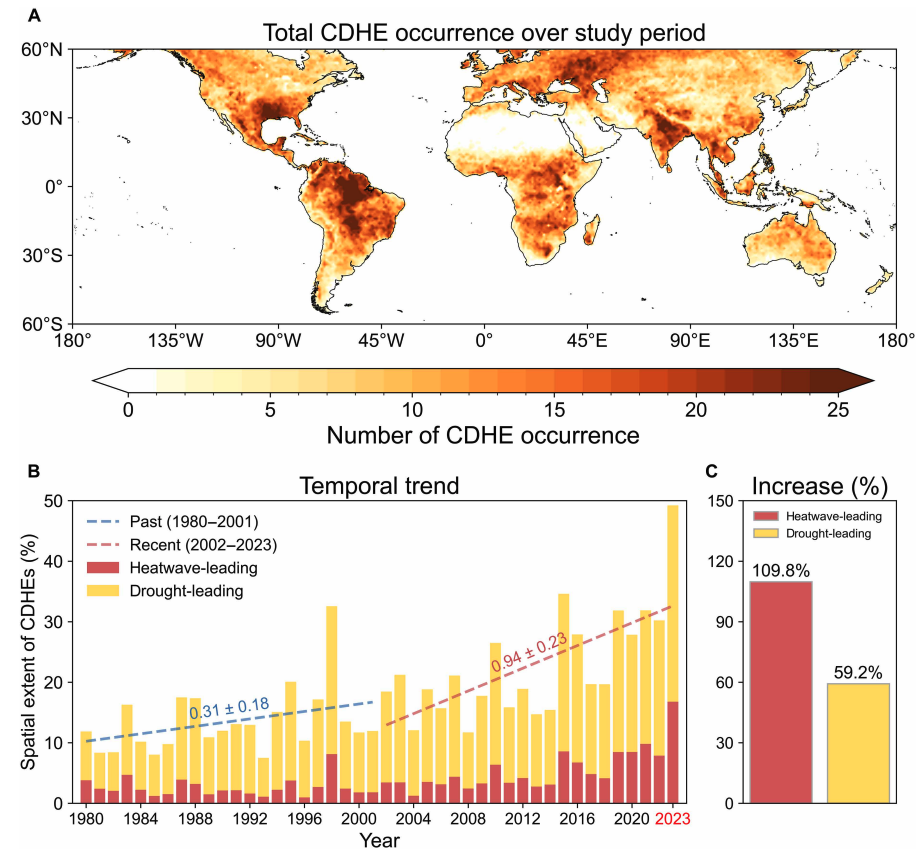
Heatwave-led events have been the main contributor to this increase, the study says, with their spatial extent rising 110% between 1980-2001 and 2002-23, compared to a 59% increase for drought-led events.
The map below shows the global distribution of CDHEs over 1980-2023. The charts show the percentage of the land surface affected by a heatwave-led CDHE (red) or a drought-led CDHE (yellow) in a given year (left) and relative increase in each CDHE type (right).
The study finds that CDHEs have occurred most frequently in northern South America, the southern US, eastern Europe, central Africa and south Asia.
Threshold passed
The authors explain that the increase in heatwave-led CDHEs is related to rising global temperatures, but that this does not tell the whole story.
In the earlier 22-year period of 1980-2001, the study finds that the spatial extent of heatwave-led CDHEs rises by 1.6% per 1C of global temperature rise. For the more-recent period of 2022-23, this increases “nearly eightfold” to 13.1%.
The change suggests that the rapid increase in the heatwave-led CDHEs occurred after the global average temperature “surpasse[d] a certain temperature threshold”, the paper says.
This threshold is an absolute global average temperature of 14.3C, the authors estimate (based on an 11-year average), which the world passed around the year 2000.
Investigating the recent surge in heatwave-leading CDHEs further, the researchers find a “regime shift” in land-atmosphere dynamics “toward a persistently intensified state after the late 1990s”.
In other words, the way that drier soils drive higher surface temperatures, and vice versa, is becoming stronger, resulting in more heatwave-led compound events.
Daily data
The research has some advantages over other previous studies, Yeh says. For instance, the new work uses daily estimations of CDHEs, compared to monthly data used in past research. This is “important for capturing the detailed occurrence” of these events, says Yeh.
He adds that another advantage of their study is that it distinguishes the sequence of droughts and heatwaves, which allows them to “better understand the differences” in the characteristics of CDHEs.
Dr Meryem Tanarhte is a climate scientist at the University Hassan II in Morocco, and Dr Ruth Cerezo Mota is a climatologist and a researcher at the National Autonomous University of Mexico. Both scientists, who were not involved in the study, agree that the daily estimations give a clearer picture of how CDHEs are changing.
Cerezo-Mota adds that another major contribution of the study is its global focus. She tells Carbon Brief that in some regions, such as Mexico and Africa, there is a lack of studies on CDHEs:
“Not because the events do not occur, but perhaps because [these regions] do not have all the data or the expertise to do so.”
However, she notes that the reanalysis data used by the study does have limitations with how it represents rainfall in some parts of the world.
Compound impacts
The study notes that if CDHEs continue to intensify – particularly events where heatwaves are the precursors – they could drive declining crop productivity, increased wildfire frequency and severe public health crises.
These impacts could be “much more rapid and severe as global warming continues”, Yeh tells Carbon Brief.
Tanarhte notes that these events can be forecasted up to 10 days ahead in many regions. Furthermore, she says, the strongest impacts can be prevented “through preparedness and adaptation”, including through “water management for agriculture, heatwave mitigation measures and wildfire mitigation”.
The study recommends reassessing current risk management strategies for these compound events. It also suggests incorporating the sequences of drought and heatwaves into compound event analysis frameworks “to enhance climate risk management”.
Cerezo-Mota says that it is clear that the world needs to be prepared for the increased occurrence of these events. She tells Carbon Brief:
“These [risk assessments and strategies] need to be carried out at the local level to understand the complexities of each region.”




The post Heatwaves driving recent ‘surge’ in compound drought and heat extremes appeared first on Carbon Brief.
Heatwaves driving recent ‘surge’ in compound drought and heat extremes
Greenhouse Gases
DeBriefed 6 March 2026: Iran energy crisis | China climate plan | Bristol’s ‘pioneering’ wind turbine
Welcome to Carbon Brief’s DeBriefed.
An essential guide to the week’s key developments relating to climate change.
This week
Energy crisis
ENERGY SPIKE: US-Israeli attacks on Iran and subsequent counterattacks across the Middle East have sent energy prices “soaring”, according to Reuters. The newswire reported that the region “accounts for just under a third of global oil production and almost a fifth of gas”. The Guardian noted that shipping traffic through the strait of Hormuz, which normally ferries 20% of the world’s oil, “all but ground to a halt”. The Financial Times reported that attacks by Iran on Middle East energy facilities – notably in Qatar – triggered the “biggest rise in gas prices since Russia’s full-scale invasion of Ukraine”.
‘RISK’ AND ‘BENEFITS’: Bloomberg reported on increases in diesel prices in Europe and the US, speculating that rising fuel costs could be “a risk for president Donald Trump”. US gas producers are “poised to benefit from the big disruption in global supply”, according to CNBC. Indian government sources told the Economic Times that Russia is prepared to “fulfil India’s energy demands”. China Daily quoted experts who said “China’s energy security remains fundamentally unshaken”, thanks to “emergency stockpiles and a wide array of import channels”.
‘ESSENTIAL’ RENEWABLES: Energy analysts said governments should cut their fossil-fuel reliance by investing in renewables, “rather than just seeking non-Gulf oil and gas suppliers”, reported Climate Home News. This message was echoed by UK business secretary Peter Kyle, who said “doubling down on renewables” was “essential” amid “regional instability”, according to the Daily Telegraph.
China’s climate plan
PEAK COAL?: China has set out its next “five-year plan” at the annual “two sessions” meeting of the National People’s Congress, including its climate strategy out to 2030, according to the Hong Kong-based South China Morning Post. The plan called for China to cut its carbon emissions per unit of gross domestic product (GDP) by 17% from 2026 to 2030, which “may allow for continued increase in emissions given the rate of GDP growth”, reported Reuters. The newswire added that the plan also had targets to reach peak coal in the next five years and replace 30m tonnes per year of coal with renewables.
ACTIVE YET PRUDENT: Bloomberg described the new plan as “cautious”, stating that it “frustrat[es] hopes for tighter policy that would drive the nation to peak carbon emissions well before president Xi Jinping’s 2030 deadline”. Carbon Brief has just published an in-depth analysis of the plan.